Draft. This book is under active development, and chapters may change. Please use ‘Report an issue’ to flag problems.
1Introduction: reproducibility as a computational problem
An article about computational science in a scientific publication is not the scholarship itself, it is merely advertising of the scholarship. The actual scholarship is the complete software development environment and the complete set of instructions which generated the figures.
Buckheit and Donoho, paraphrasing Jon Claerbout, WaveLab and Reproducible Research (1995)
1.1 A result that ran only once
Every quantitative health scientist has met the failure this book exists to prevent. An analysis runs cleanly on the machine where it was written and produces a table, a figure, a p-value. A year later, on a new laptop, or a colleague’s, or a reviewer’s, the same code errors. Worse, it may run to completion and return a different number. The statistics were sound. What failed was everything around the statistics: a package that changed beneath the code, a default that shifted between releases of R, a system library present on one machine and absent on another. The result had been reproducible exactly once, on one machine, at one moment, and no one noticed until the moment had passed.
This book is about closing that gap. Its subject is computational reproducibility, by which we mean the property that a computational result can be regenerated, within a stated tolerance, by another person on another machine at a later time. That is a narrower claim than scientific replication, and we shall be careful to keep the two apart throughout. It is nonetheless a claim that a great deal of published health-sciences research cannot currently support. Unlike replication, it is also a claim that can be secured by technical means available today.
We begin by fixing the vocabulary of the field and then review the evidence that computational reproducibility is often not achieved. We then consider why the failures are computational in character, and introduce the tools and the framework that the book uses. Lastly, we set out the plan of the book and how it is meant to be used.
1.2 What reproducibility means
The vocabulary of this field is contested, and the reader should fix the terms before wading into the literature. We follow the distinction adopted by the National Academies in their 2019 consensus report (National Academies of Sciences, Engineering, and Medicine, 2019). Reproducibility is obtaining consistent computational results using the same input data, computational steps, methods, code, and conditions of analysis. That is, it is a statement about re-execution. Replicability is obtaining consistent results across studies aimed at answering the same question, each with its own data. It is a statement about whether a scientific finding holds on new data. The two are independent. A result can be perfectly reproducible and entirely wrong, if the code faithfully regenerates a mistaken number every time. Conversely, a finding can replicate across laboratories while no single analysis in the set is computationally reproducible. Leek and Peng press the point that a reproducible analysis can still be wrong, and that reproducibility is therefore a floor rather than a ceiling (Leek & Peng, 2015). This book concerns itself almost entirely with the first of the two terms, and we say so plainly wherever the boundary is in doubt.
Reproducibility so defined is a spectrum. Peng (2011) arranged computational work along a scale from the merely published, through code available, code and data available, and linked and executable, to fully replicable. He argued that ‘reproducibility has the potential to serve as a minimum standard for judging scientific claims when full independent replication of a study is not possible’. We take from Peng the idea that reproducibility comes in degrees, and that honesty about which degree one has reached is itself a scientific virtue. We shall develop that idea into the levels ladder of Chapter 3.
1.3 The evidence that it is not happening
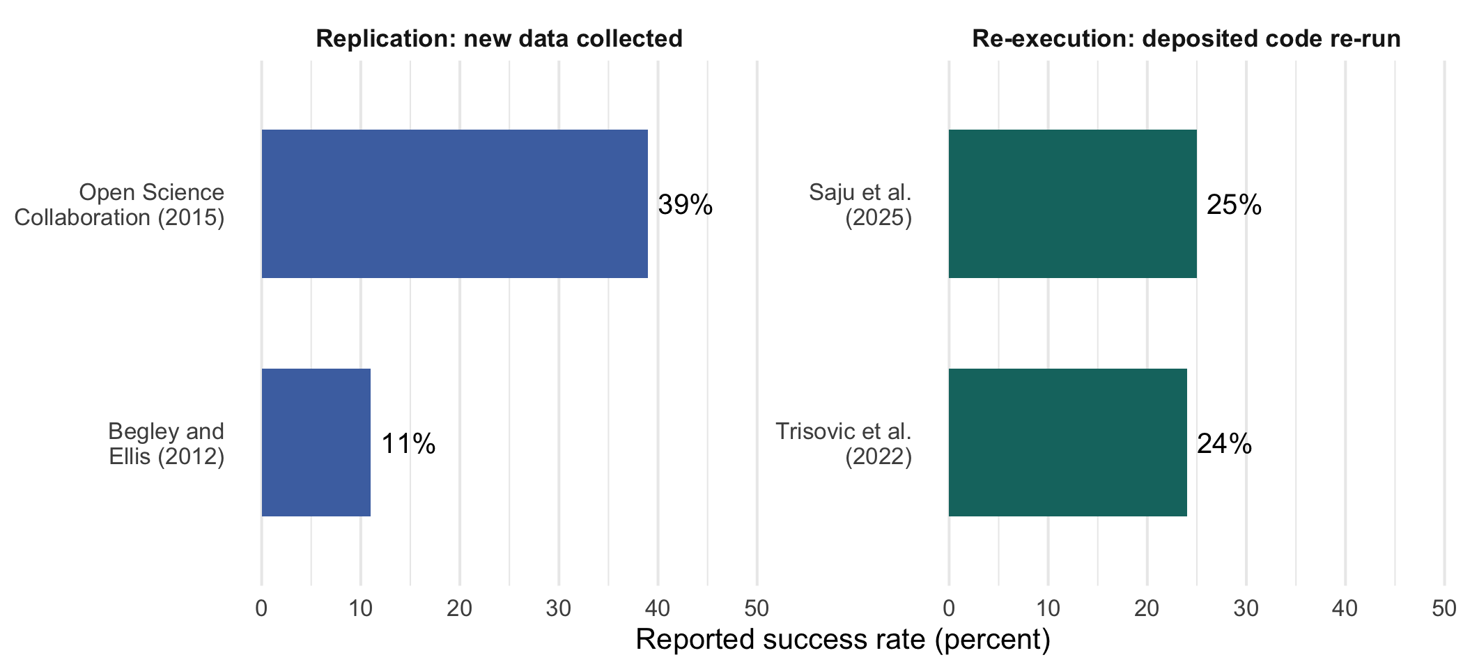
The case for taking this seriously is empirical, and it is grim. In psychology, the Open Science Collaboration’s teams judged only 39 of 100 replications successful (Open Science Collaboration, 2015). In preclinical oncology, Begley & Ellis (2012) reproduced only 6 of 53 landmark findings. These are replication failures, at the scientific end of the spectrum, and their causes are many. However, a growing body of evidence isolates the specifically computational failures. These are, if anything, more damning, because they are more avoidable.
Trisovic et al. (2022) re-ran more than nine thousand R files deposited in the Harvard Dataverse. They found that roughly one in four executed without error, and that was before asking whether the output matched. Saju et al. (2025), examining R code supplements on the Open Science Framework, found that only about a quarter of the R scripts ran without error, even after an automated pipeline rebuilt their environments. They also found that nearly every project carried no description of its dependencies at all. These analyses could not be made to run a second time, so the question of whether they reached the right conclusion never arose. The scholarship, in Buckheit and Donoho’s paraphrase of Claerbout, was advertised but never delivered.
Setting the four studies beside one another, as in Figure 1.1, makes the shape of the problem visible. The replication studies and the re-execution studies measure different things, and for that reason the figure keeps them in separate panels. Nevertheless, the rates are comparably low in both. The right-hand panel differs in one respect: it counts failures that better engineering would fix and that no amount of additional data collection would.
library(ggplot2)library(tibble)studies<-tibble( study =c('Open Science\nCollaboration (2015)','Begley and\nEllis (2012)','Trisovic et al.\n(2022)','Saju et al.\n(2025)'), rate =c(39, 11, 26, 26), kind =factor(c('Replication: new data collected','Replication: new data collected','Re-execution: deposited code re-run','Re-execution: deposited code re-run'), levels =c('Replication: new data collected','Re-execution: deposited code re-run')))ggplot(studies, aes(x =reorder(study, rate), y =rate))+geom_col(aes(fill =kind), width =0.62, show.legend =FALSE)+geom_text(aes(label =paste0(rate, '%')), hjust =-0.18, size =3.4)+coord_flip(ylim =c(0, 48))+facet_wrap(~kind, scales ='free_y', ncol =2)+scale_fill_manual(values =c('Replication: new data collected'='#4c72b0','Re-execution: deposited code re-run'='#14746f'))+labs(x =NULL, y ='Reported success rate (percent)')+theme_minimal(base_size =10)+theme( panel.grid.major.y =element_blank(), strip.text =element_text(face ='bold', size =8.5))
Figure 1.1: Reported success rates in four studies, separated by what each measured. The left panel reports replication studies, in which new data was collected to test a prior finding. The right panel reports re-execution studies, in which deposited code was run again without any attempt to evaluate the science. The re-execution figures are those stated in the text of the studies as cited in this chapter, and are approximate where the source reports a bound rather than a point estimate.
The figure tells us how often replication and re-execution fail. It does not tell us why, and that question is taken up next.
1.4 Why the failures are computational, not statistical
The reasons re-execution fails point directly at the remedy. Consider two changes to R itself, each silent and each capable of altering a published result. In R 3.6.0 the default algorithm that sample() uses to turn a seed into draws changed. Code that set a seed and drew a sample therefore obtained different draws before and after the release, with no error and no warning. In R 4.0.0 the stringsAsFactors default flipped from TRUE to FALSE. Code reading a data frame then silently produced character columns where it once produced factors. Any code that depended on factor-specific behavior, such as the ordering of levels or a function that requires a factor, behaved differently as a result. Neither change was a bug; both were improvements. Both would nonetheless break the exact reproduction of an analysis written under the old default, and neither would announce itself.
These are instances of a general phenomenon. A computational result depends not only on the code and the data but on a stack of determinants beneath them. The stack includes the operating system and its system libraries, the numerical libraries that implement linear algebra, the language runtime, the exact versions of every package, and the session configuration. That configuration includes the random-number kind, the contrasts, the number of printed digits, and the locale and time zone. Underneath all of it sits the hardware. A published script pins almost none of these. It records the analysis logic and, if the reader is fortunate, the data. The remaining layers are left to whatever the next machine happens to provide. Reproducibility fails in the gap between what the script fixes and what the result depends on, and the task of a reproducibility toolchain is to close that gap, layer by layer. But how far down the stack has a given effort actually reached? That is the organizing question of this book.
1.5 The tools, and the framework this book uses
The R ecosystem has, over two decades, produced mature tools for nearly every layer of that stack. Literate programming, through knitr, R Markdown, and now Quarto (Allaire et al., 2024), binds prose to the code that produces it. renv(Ushey & Wickham, 2026) pins package versions in a lockfile. Docker, through Rocker’s R-specific base images (Boettiger, 2015; Nüst et al., 2020), pins the operating system and its libraries. Continuous integration re-runs the whole compendium on a clean machine to confirm that the pinned layers actually suffice. Alternatives exist at every layer: Nix and its R front-end rix in place of renv(Dolstra et al., 2004; Rodrigues & Baumann, 2024), Podman or Apptainer in place of Docker (Kurtzer et al., 2017), GitLab in place of GitHub. We introduce each tool where the chapter ahead needs it, not in one early catalog. Package pinning appears in Chapter 6, and the environment and its alternatives in Chapter 7 and Chapter 8. Chapter 5 treats the compendium structure that Gentleman & Temple Lang (2007) and Marwick et al. (2018)’s rrtools established. Finally, Chapter 10, Chapter 11, and Chapter 12 treat the workflow, quality, and validation layer.
The difficulty lies in composing this tooling by hand. renv says nothing about the operating system, and Docker says nothing about which package versions are installed inside it. Neither says anything about session configuration. A researcher who wants a genuinely reproducible analysis must therefore assemble all of it correctly, for every project, by hand. The running example of this book uses zzcollab, a framework that assembles the triad (renv for packages, Docker for the environment, continuous integration for validation) into one workflow. A biostatistician thereby obtains the composition without building it from scratch. Each chapter ahead develops the part of zzcollab relevant to its own layer, against the concept it has just introduced.
Like every tool this book covers, zzcollab is held to the standard it teaches. By its own accounting it firmly pins a part of the determinant stack, namely the environment, the packages, the source, and the locale and time zone. It leaves the rest (the numerical libraries, the random-number discipline, the graphics device, intrinsic non-determinism) to the base image or to convention. Reproducibility tooling in general has an adoption problem more than a capability problem. Saju et al. (2025) found that most deposited code supplements carry no dependency description at all, even though mature, free, documented tools for that exact problem have existed for years. The task of this book is therefore to make existing capability teachable and routine. It is also to state plainly, at each level of the ladder, what a given effort has secured and what remains exposed, including its own.
1.6 The plan of this book
The book is organized in four parts, and three ideas recur in every chapter. The first is the ladder of reproducibility levels (L0 locatable, L1 pinned packages, L2 pinned environment, L3 verified), which we introduce in Chapter 3 and use thereafter as the common scale. The second is the distinction between capturing reproducibility and validating it. That is, pinning is capture, while continuous integration and verification are validation. The third is the research compendium as the unit of reproducible work, introduced in Chapter 5. The book is written for a one-quarter, ten-week course. Not every chapter fits in ten weeks, and an instructor teaching on that schedule should expect to treat some material as optional. The four parts proceed as follows.
Part I, Foundations. The reproducibility crisis and its computational character (Chapter 2); the levels of reproducibility and the determinants that set them (Chapter 3); version control with git as the foundation of a locatable analysis (Chapter 4); and the research compendium (Chapter 5).
Part II, Capturing the environment. Pinning packages with a lockfile (Chapter 6); pinning the operating system and runtime with a container (Chapter 7); and the alternatives, from Nix to Podman to Apptainer (Chapter 8).
Part III, Validation. The practices that let a pinned analysis be re-run and checked: literate programming and the rendered report (Chapter 9); automating the analysis with make and targets (Chapter 10); testing and code quality (Chapter 11); and continuous integration and verification (Chapter 12).
Part IV, Collaboration and stewardship. Sharing a compendium with a team and with the world (Chapter 13).
1.7 How to use this book
The book is meant to be worked, not only read. Each chapter develops a concept and then builds it, in R and at the shell, inside a running example compendium. The reader who follows along will finish with a reproducible project of their own. More durably, the reader will acquire the judgment to reason about reproducibility with any toolchain, and to state without flinching the level a given analysis has actually reached.
Seven habits recur across the chapters that follow. A chapter’s own rules of thumb will cite a habit by number rather than restate it. The closing chapter recalls them once the argument of the book is complete.
NoteSeven habits, and a motto
Claim only the level you have verified.
Commit before you compute.
Pin what you ran, not what is current.
Never commit, deposit, or paste restricted data.
Make every gate able to fail, and watch it fail once.
Compare against a recorded baseline, with a stated tolerance.
Rebuild from clean, on a machine that is not yours.
Write the honest level down.
Allaire, J. J., Teague, C., Scheidegger, C., Xie, Y., & Dervieux, C. (2024). Quarto: An open-source scientific and technical publishing system. https://quarto.org/
Begley, C. G., & Ellis, L. M. (2012). Raise standards for preclinical cancer research. Nature, 483(7391), 531–533. https://doi.org/10.1038/483531a
Boettiger, C. (2015). An introduction to docker for reproducible research. ACM SIGOPS Operating Systems Review, 49(1), 71–79. https://doi.org/10.1145/2723872.2723882
Dolstra, E., Jonge, M. de, & Visser, E. (2004). Nix: A safe and policy-free system for software deployment. Proceedings of the 18th USENIX Conference on System Administration (LISA ’04), 79–92.
Gentleman, R., & Temple Lang, D. (2007). Statistical analyses and reproducible research. Journal of Computational and Graphical Statistics, 16(1), 1–23. https://doi.org/10.1198/106186007X178663
Kurtzer, G. M., Sochat, V., & Bauer, M. W. (2017). Singularity: Scientific containers for mobility of compute. PLOS ONE, 12(5), e0177459. https://doi.org/10.1371/journal.pone.0177459
Leek, J. T., & Peng, R. D. (2015). Reproducible research can still be wrong: Adopting a prevention approach. Proceedings of the National Academy of Sciences, 112(6), 1645–1646. https://doi.org/10.1073/pnas.1421412111
Marwick, B., Boettiger, C., & Mullen, L. (2018). Packaging data analytical work reproducibly using R (and friends). The American Statistician, 72(1), 80–88. https://doi.org/10.1080/00031305.2017.1375986
National Academies of Sciences, Engineering, and Medicine. (2019). Reproducibility and replicability in science. The National Academies Press. https://doi.org/10.17226/25303
Nüst, D., Eddelbuettel, D., Bennett, D., Cannoodt, R., Clark, D., Daroczi, G., Edmondson, M., Fay, C., Hughes, E., et al. (2020). The Rockerverse: Packages and applications for containerisation with R. The R Journal, 12(1), 437–461. https://doi.org/10.32614/RJ-2020-007
Open Science Collaboration. (2015). Estimating the reproducibility of psychological science. Science, 349(6251), aac4716. https://doi.org/10.1126/science.aac4716
Rodrigues, B., & Baumann, P. (2024). Rix: Reproducible data science environments with Nix. https://docs.ropensci.org/rix/
Saju, L. et al. (2025). Computational reproducibility of R code supplements on OSF. arXiv Preprint arXiv:2505.21590. https://arxiv.org/abs/2505.21590
Trisovic, A., Lau, M. K., Pasquier, T., & Crosas, M. (2022). A large-scale study on research code quality and execution. Scientific Data, 9(1), 60. https://doi.org/10.1038/s41597-022-01143-6