Sandve, Nekrutenko, Taylor, and Hovig, Ten Simple Rules for Reproducible Computational Research, Rule 2 (2013)
10.1 Learning objectives
By the end of this chapter the reader should be able to:
Diagnose the failure mode of a manually run, multi-step analysis: steps run out of order, an upstream change leaves a downstream output stale, and no one can be sure the whole thing still runs end to end from raw data to report.
Express an analysis as a directed acyclic graph of steps, and explain why a single command can then rebuild exactly what is out of date and nothing more.
Read and write a GNU Make rule, its target, prerequisites, and recipe, explain the timestamp-based staleness check, and say why Make’s reach is language-agnostic.
Build an R-native, function-oriented pipeline with targets: the _targets.R script, tar_target, tar_make, and tar_visnetwork, and explain how targets invalidates exactly the targets that depend on a changed function, object, or package.
State, in the book’s capture-versus-validation terms, precisely what a pipeline does and does not add to the reproducibility ladder.
Judge how heavily the pipeline machinery bears on each research archetype, and name the language-agnostic managers, Snakemake and Nextflow, and workflowr, for readers whose work reaches beyond R.
10.2 Orientation
Consider an analysis that has grown, as most do, one step at a time. There is a script that reads the raw export and writes a cleaned dataset. A second fits a model to the cleaned data and saves the fitted object. A third draws the figures from the model, and a report assembles the figures and the tables into a manuscript. Each script runs, and the analyst runs them in order, by hand, at the console. For a while this works.
The trouble begins when the raw data are corrected. The analyst re-runs the cleaning script, and now must remember three further things: that the model depends on the cleaned data and must be re-run, that the figures depend on the model and must be re-run, and that the report depends on the figures and must be re-rendered. Each of these is a separate act of memory. Miss one, and the report now shows a figure drawn from the old model, fitted to the old data, and nothing in the document announces the discrepancy. The output is stale: it is downstream of a change that never propagated to it. Worse, the staleness is invisible, because a stale figure is a perfectly valid PNG file that opens and displays without complaint.
This is the failure this chapter exists to prevent, and it has three faces. The first is order: the steps have a required sequence, cleaning before modeling before plotting, and running them out of order produces either an error or, more dangerously, a result computed from the wrong inputs. The second is staleness: a change to an upstream file leaves every downstream output obsolete, and re-propagating the change by hand is exactly the kind of bookkeeping a human does poorly. The third is the end-to-end doubt. After a session of editing scripts and re-running some of them, the analyst cannot honestly say whether the whole analysis still runs from raw data to finished report. It has been weeks since anyone ran it all, in order, in one act. The project works, in the sense that its outputs exist, but no one can be sure it would work if rebuilt from nothing.
The remedy is to stop treating the analysis as a remembered sequence of commands and to express it instead as a structure: a graph of steps, each declaring what it consumes and what it produces, from which a machine can work out the order, detect the staleness, and re-run exactly what a change requires. That structure is a pipeline, and this chapter is about two tools that build one, the venerable and language-agnostic GNU Make and the R-native targets. The manual-steps critique that motivates them is stated crisply in the practices literature: Sandve et al. (2013), in their second rule, urge that one ‘avoid manual data manipulation steps’ and automate the path from raw data to result, precisely because a manual path cannot be trusted to have been followed the same way twice.
10.3 The analyst’s contribution
Three judgments in this chapter are the analyst’s own, and no pipeline tool makes them.
Deciding where the steps divide. A pipeline is a graph of steps, and the analyst chooses what a step is: how finely to cut the analysis into targets, which computations to group and which to separate. Cut too coarsely, into one enormous step, and the pipeline caches nothing useful, because any change re-runs everything. Cut too finely, into hundreds of trivial targets, and the graph becomes hard to read and the bookkeeping overhead dominates. The right granularity puts the expensive, stable computations, a model fit, a simulation run, in targets of their own, so that a change elsewhere does not needlessly re-run them. This is a design decision, and it trades caching benefit against graph legibility.
Keeping the dependency declarations honest. A pipeline can only track dependencies it is told about, or can infer. Make infers nothing; every prerequisite an analyst omits from a rule is a dependency the tool cannot see, and an omitted prerequisite is exactly how a stale output slips through. targets infers a great deal automatically, but it too can be defeated, by a step that reads a file without declaring it as a file target, or that reaches for global state the tool cannot trace. Getting the declared dependencies to match the real ones is the analyst’s responsibility, and it is the single discipline on which a pipeline’s correctness rests.
Matching the claim to what a pipeline delivers. A pipeline mechanises re-execution. It does not pin a package, fix an environment, or establish that a result is correct. An analyst who says ‘the analysis is reproducible’ because tar_make() runs to completion has claimed more than the pipeline delivers, in exactly the way, and for exactly the reasons, that the sealed render of Chapter 9 is not by itself a reproducibility guarantee. The pipeline secures the act of re-running; the level reached is a separate question, settled by the lockfile, the container, and the verification of the later chapters.
NoteThe vocabulary of this chapter
Pipeline. An analysis expressed as a set of steps, each declaring its inputs and outputs, so that the whole can be re-executed by a single command that runs the steps in dependency order.
Dependency graph. The graph whose nodes are the steps and whose edges record that one step consumes what another produces. A valid pipeline’s graph is a directed acyclic graph (DAG): directed because inputs flow to outputs, and acyclic because a step cannot, directly or transitively, depend on its own output.
Target. A single step in the pipeline, together with the output it produces. The word is shared by Make and targets, with a shift of emphasis: for Make a target is a file, for targets it is more often an R object.
Prerequisite. In Make, an input a target depends on. If any prerequisite is newer than the target, the target is out of date.
Recipe (or command). The shell command Make runs to bring a target up to date from its prerequisites.
Staleness (out-of-date). The condition of a target whose inputs have changed since it was last built, so that its stored output no longer reflects its inputs.
Up-to-date (skippable). The condition of a target whose inputs have not changed since it was last built, so that rebuilding it would reproduce the stored output and can be skipped.
Invalidation. The act of marking a target out of date because something it depends on, a file, an upstream target, a function, or a package, has changed.
10.4 The analysis as a dependency graph
The conceptual move that a pipeline asks of an analyst is to stop thinking of the analysis as a list of commands to run and to start thinking of it as a graph of dependencies to satisfy. The two descriptions contain the same steps, but they license different machinery. A list of commands can only be replayed, from the top, every time. A graph of dependencies can be interrogated, so that a tool can answer the question a list cannot, which steps actually need to run now, given what has changed?
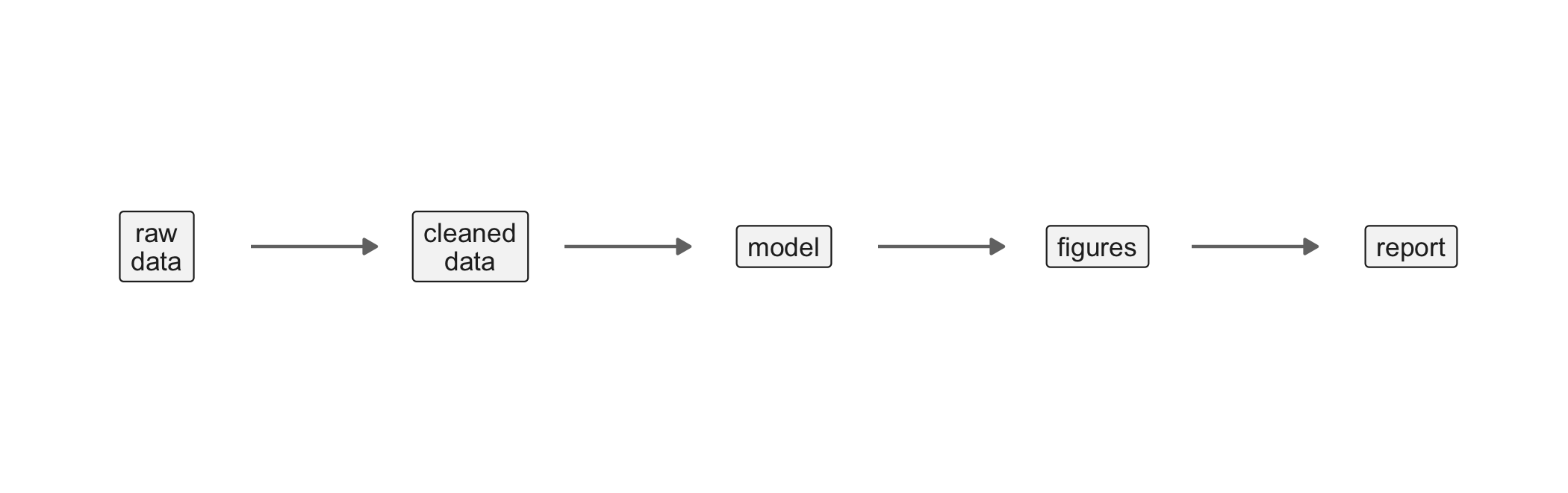
Figure 10.1 draws the graph for the small analysis of the orientation. Each node is a step that produces an output, and each arrow records that the step at its head consumes what the step at its tail produces. The graph is directed, because the flow from raw data to report has a direction, and it is acyclic, because no output feeds, however remotely, back into its own inputs. This is the directed acyclic graph, the DAG, that every pipeline tool builds internally, whether or not it draws it for you.
Figure 10.1: The analysis of the orientation as a directed acyclic graph. Each node is a step that produces an output; each arrow records that the step it points to consumes what the previous step produced. A change to the raw data invalidates every node downstream of it (all four to its right); a change to the plotting code invalidates only the figures and the report. A pipeline tool reads this graph to rebuild exactly the stale nodes and skip the rest.
Two operations on this graph are the whole point of a pipeline. The first is the topological sort: reading the arrows, the tool can order the steps so that no step runs before the steps it depends on, which is the order the analyst was keeping in their head and now need not. The second is selective rebuild: given a record of what each step last consumed, the tool can mark a step stale when any of its inputs has changed and up to date otherwise, and then rebuild only the stale steps and those downstream of them. If the raw data change, all four downstream nodes are stale and all four rebuild. If only the plotting code changes, the figures and the report are stale but the cleaned data and the model are not, and the model, which may have taken an hour to fit, is not re-fitted. The single command that triggers this, make or tar_make(), replaces the remembered sequence with one reliable act, and the end-to-end doubt of the orientation is dissolved, because the one act, by construction, runs everything that is out of date and leaves nothing behind.
10.4.1 The graph of an actual analysis
Figure 10.1 draws the shape in the abstract. It is worth seeing the same shape over an analysis that runs, because a real graph is less tidy than a diagram and the untidiness is where the argument lives.
library(tibble)library(knitr)time_it <-function(expr) { t <-system.time(force(expr))[['elapsed']]round(1000* t, 1)}d <- survival::diabetict_load <-time_it(d <- survival::diabetic)t_clean <-time_it({ d$arm <-factor(d$trt, levels =c(0, 1),labels =c('Untreated', 'Laser')) d <- d[!is.na(d$time), ]})t_fit <-time_it( fit <- survival::coxph(survival::Surv(time, status) ~ arm + age,data = d))t_boot <-time_it({set.seed(1)replicate(200, { i <-sample(nrow(d), replace =TRUE)unname(coef(survival::coxph( survival::Surv(time, status) ~ arm + age, data = d[i, ]))[1]) })})steps <-tibble(Step =c('read raw data', 'derive arm labels','fit proportional-hazards model','bootstrap the treatment effect'),`Consumes`=c('--', 'raw data', 'cleaned data','cleaned data'),`Elapsed (ms)`=c(t_load, t_clean, t_fit, t_boot))kable(steps, align ='llr')
Table 10.1: The retinopathy analysis expressed as a dependency graph, with the cost of each step measured rather than asserted. The timings are from one run on one machine and will differ on another; their ratios are the durable part. Note that the two expensive steps sit at the end, so an edit to the plotting code that forced a full rebuild would waste almost all of the total.
Step
Consumes
Elapsed (ms)
read raw data
–
0
derive arm labels
raw data
0
fit proportional-hazards model
cleaned data
6
bootstrap the treatment effect
cleaned data
305
The measured ratios make the argument that prose cannot. On this build the bootstrap costs about 51 times the model fit, and the two steps above it are too fast to measure at all, so the value of selective rebuild is not a matter of taste: an analyst who re-runs everything after changing a label pays for the bootstrap to learn nothing. That ratio is itself an inline expression, for the reason Chapter 9 gives; had it been typed, the next machine to build the book would have made it false.
It is also the case for a cache with a caveat, and the caveat is this table itself. These timings are computed when the book is built, so they describe the build machine and not the reader’s, and a slower machine would show different absolute values. The ratio between the last row and the others is what survives, which is the same distinction the verification chapter draws between a result worth recording and a measurement worth repeating.
10.5 GNU Make: targets, prerequisites, and rules
The oldest and most widely used pipeline tool is GNU Make, a reimplementation of the make utility first written in 1976 to compile programs and pressed into service for data analysis ever since. Make is worth learning first, before any R-specific tool, for two reasons: its model is the simplest possible expression of the pipeline idea, so that understanding it is understanding pipelines in general; and its reach is language-agnostic, so that a single Makefile can orchestrate an analysis whose steps are written in R, Python, the shell, and a typesetting engine, without knowing or caring what language each step uses.
A Makefile is a list of rules, and a rule has three parts: a target, the file the rule produces; its prerequisites, the files the target depends on, written after a colon; and a recipe, the shell command that builds the target from its prerequisites, written on the following line and, by an unforgiving convention, indented with a literal tab. The analysis of Figure 10.1 becomes four rules:
Read the rules from the bottom up and the dependency graph is plain: cleaned.rds depends on the cleaning script and the raw data; model.rds depends on the fitting script and the cleaned data; and so on up to the report. Make never has to be told the order, because the order is implied by the prerequisites. It reads the whole Makefile, builds the graph, sorts it, and knows that cleaned.rds must be built before model.rds because the latter names the former as a prerequisite. To rebuild the analysis the analyst types a single command:
make report.html
or, since the first target in the file is the default, simply make. Make walks the graph and rebuilds what is needed, in order, and reports each recipe as it runs.
The mechanism by which Make decides what is needed is the one subtlety worth dwelling on, because it is both the source of Make’s power and the source of its most common surprise. Make is timestamp-based. It compares the modification time of each target against the modification times of its prerequisites, and it considers a target out of date if any prerequisite is newer than the target. Edit fit_model.R, and its modification time advances past that of model.rds; Make sees that model.rds is now older than a file it depends on, rebuilds it, which advances the timestamp of model.rds past that of figures.rds, and so the rebuild propagates downstream exactly as far as the change reaches and no further. A target all of whose prerequisites are older than it is already up to date, and Make skips it, printing a line to the effect that there is nothing to be done. This is the selective rebuild of the previous section, implemented with nothing more than the file system’s clock.
The timestamp rule is also Make’s principal limitation, and an honest account must state it. Make knows only whether a file is newer, not whether its contents have changed. Touching a file without editing it will trigger a needless rebuild, and, more subtly, a change that does not alter a file’s modification time will be missed. Make also tracks only what the analyst declares. It has no way to know that fit_model.R reads a configuration file unless that file is listed as a prerequisite; an undeclared input is invisible, and its change will not trigger the rebuild it should. And Make tracks files and only files: it cannot cache an in-memory R object, so every step must serialize its result to disk, and the graph is a graph of files. These limitations are the opening that the R-native tools were built to close.
NoteCheck your understanding: what Make rebuilds
A project uses the four-rule Makefile above. The analyst edits make_figures.R to change a color palette and runs make. Which of the four targets does Make rebuild, and which does it skip? Explain your answer in terms of the timestamp rule.
NoteAnswer
Editing make_figures.R advances its modification time past that of figures.rds, so figures.rds is now older than one of its prerequisites and Make rebuilds it. Rebuilding figures.rds advances its timestamp past that of report.html, so report.html is rebuilt too. Make skips cleaned.rds and model.rds: neither the raw data, the cleaning script, the fitting script, nor the cleaned data changed, so each of those targets remains newer than all of its prerequisites and is up to date. The expensive model fit is not repeated, which is the payoff of expressing the analysis as a graph.
10.6 targets: a function-oriented pipeline for R
Make treats an analysis as a graph of files built by shell commands. For an R analysis this is a slightly awkward fit: every step must be a script that reads files and writes files, the intermediate objects must all be serialized to disk by hand, and Make’s timestamp check is blind to the thing an R analyst most wants tracked, the R functions that do the work. The targets package, written by William Landau as the successor to his earlier drake(Landau, 2018, 2021), reworks the pipeline idea natively for R and closes exactly these gaps.
The reframing is captured in the phrase ‘function-oriented’. In a targets pipeline the analyst writes the analysis as a set of R functions, one for each meaningful step, and then declares, in a special script named _targets.R at the project root, a list of targets that connect those functions into a graph. Each target is created by tar_target(), which names the target and gives the R expression that produces it. Targets reads those expressions, notices that one target’s expression mentions another target’s name, and infers the dependency graph automatically, with no colons and no prerequisites to maintain by hand. A _targets.R for our running analysis reads:
library(targets)tar_option_set(packages =c('dplyr', 'ggplot2'))# Analysis functions live in R/ and are sourced here.tar_source('R')list(tar_target( raw_file,'data/raw_data.csv',format ='file' ),tar_target(raw_data, read_raw(raw_file)),tar_target(cleaned, clean_data(raw_data)),tar_target(model, fit_model(cleaned)),tar_target(figures, make_figures(model, cleaned)),tar_target( report,render_report(model, figures),format ='file' ))
Several features distinguish this from the Makefile, and each is the point. The intermediate results, raw_data, cleaned, model, figures, are R objects, not files. targets stores each in a hidden _targets/ store, keyed and versioned, and hands it to the next target as a plain R value. The analyst never writes a saveRDS or a readRDS, because the storage is the tool’s job. Where a real file must be tracked, the raw CSV at the top and the rendered report at the bottom, the target is declared with format = 'file', and targets then watches the file’s contents, by hashing them, rather than the R object.
That hashing is the second and deeper difference. Where Make compares timestamps, targets compares content hashes, so that a file touched but not changed does not trigger a rebuild, and a change that leaves the timestamp untouched is nonetheless caught. And the hashing extends past the data to the code: targets records a hash of the body of every function a target calls, and of the R expression in the target itself, so that editing fit_model() invalidates the model target, and everything downstream of it, even though no file has changed at all. This is what Make cannot do. A changed function invalidates exactly the targets that use it, directly or transitively, and no others; a change to make_figures() invalidates figures and report but leaves model untouched, and the expensive fit is preserved. Sensitivity to the versions of the packages a target loads is a separate matter, and one that targets does not provide: tar_option_set(packages = ...) merely attaches those packages to each target’s evaluation environment, as a call to library() would, and by default targets does not track a package’s version or invalidate a target when that version changes. Version-sensitivity comes from the lockfile of Chapter 6, which is why Landau recommends renv alongside targets rather than in place of it.
Two commands drive the pipeline. To see the graph, tar_visnetwork() draws it as an interactive network, coloring each target by whether it is up to date or out of date, which is Figure 10.1 made live and queryable:
tar_visnetwork()
To run the pipeline, tar_make() walks the graph, in a fresh R session, and builds every target that is out of date while skipping every target that is up to date:
tar_make()
On the first run every target builds and targets reports each in turn. Edit make_figures() and run tar_make() again, and the output is eloquent: targets reports that figures and report are built and that raw_data, cleaned, and model are skipped, each marked as already current. The analyst did not have to remember which steps the edit affected; the tool derived it from the graph and the hashes. And a companion command, tar_outdated(), answers the end-to-end doubt directly, by listing the targets that a tar_make() would rebuild without running anything, so that one can ask, at any moment, ‘what is stale?’ and get an exact answer.
NoteCheck your understanding: what targets tracks that Make does not
In the Makefile, editing the body of a function used by fit_model.R without changing any file’s dependency declaration might not trigger a rebuild of the downstream targets. Explain why targets does trigger it, and name the two things targets hashes that Make does not.
NoteAnswer
Make decides staleness by comparing file modification times against declared prerequisites, so a change that is not reflected in a listed prerequisite’s timestamp is invisible to it. targets instead hashes the contents of its inputs and, crucially, the bodies of the functions each target calls and the R expression in the target itself. Editing the function body changes its hash, which invalidates every target that calls it and everything downstream, so the rebuild propagates correctly. The two things targets hashes that Make does not are the R function definitions and the in-memory R objects (rather than only on-disk files), which together let it track code changes and object changes that a timestamp comparison cannot see.
10.7 What a pipeline does, and does not, add
It is worth stating with care what a pipeline contributes to reproducibility, because the answer is easily overstated in one direction and undersold in the other, and the book’s capture-versus-validation framework makes the precise statement available.
Recall the framework. A computational result depends on a stack of determinants, the operating system, the system libraries, the R version, the package versions, the session configuration, the data, the source, and reproducibility is secured by capturing each determinant, which is what a lockfile and a container do, and validating that the capture suffices, which is what continuous integration and verification do. The ladder, L0 locatable, L1 pinned packages, L2 pinned environment, L3 verified, measures how far down the stack an effort has reached.
Against this framework the pipeline occupies a precise and initially surprising position: a pipeline captures no new determinant and adds no rung to the ladder. It does not pin a package version; that is the lockfile’s work, unchanged by whether a pipeline exists. It does not fix an environment; that is the container’s. It does not verify that an output is correct; that is verification’s. An analysis run through targets and an identical analysis run by hand, on the same machine, with the same packages, produce the same numbers and sit at the same level of the ladder. In the strict accounting of determinants, the pipeline changes nothing.
Yet it would be wrong to conclude that the pipeline is reproducibility-neutral, and the reason returns us to the distinction that organizes the book. What a pipeline does is mechanize the re-execution that validation depends on. Verification, in Chapter 12, checks that rebuilding the analysis from its captured inputs reproduces the recorded outputs; continuous integration runs that rebuild on every change, in a clean machine. Both presuppose that ‘rebuild the analysis’ is a single, reliable, complete act, and it is precisely that act which a manually run analysis cannot guarantee, because the human running it may re-run some steps and forget others. The pipeline turns ‘rebuild the analysis’ from a remembered sequence into one command whose completeness is structural rather than remembered, and in doing so it removes the ‘did I re-run everything?’ doubt that is the quiet enemy of every validation step. A pipeline is thus to re-execution what continuous integration is to checking: it captures no determinant and adds no rung, but it makes the re-execution that verification (Chapter 12) confirms reliable and repeatable.
The relation to continuous integration is especially close, and worth making explicit, because the two are sometimes confused. Continuous integration is the machine that is not yours, running the rebuild in a clean environment on every change; the pipeline is the definition of what ‘the rebuild’ means. They compose naturally: a CI workflow’s core step, for a pipelined project, is to restore the environment and then run tar_make() or make, so that the pipeline supplies the re-execution and CI supplies the clean, automatic, external trigger for it. Neither replaces the other. The pipeline without CI still requires a human to remember to run it; CI without a pipeline must hard-code the sequence of steps that the pipeline would have derived from the graph. Together they close the loop: a change is pushed, a clean machine rebuilds exactly what the change made stale, and the result is checked, with no act of memory anywhere in the chain.
ImportantThe honest level
A pipeline that runs to completion demonstrates that the analysis re-executes as a single act. It does not demonstrate that the packages are pinned (L1), that the environment is fixed (L2), or that the outputs are correct and verified (L3). tar_make() succeeding is a statement about re-execution, not about level. Match the claim to the level actually reached: the pipeline secures the how of rebuilding, and the lockfile, the container, and the verification command secure the what that is rebuilt into.
10.8 Pipelines across the archetypes
As with every tool in this book, the weight the pipeline machinery carries varies sharply across the research archetypes, and a reader whose mental image is fixed on one archetype will misjudge how much of this chapter applies to another.
For the data-analysis archetype the pipeline is at its most valuable. Such a project is a chain of transforms from a raw export to a set of results for a decision, run and re-run many times as the data are corrected, the cleaning is refined, and the model is adjusted. It is exactly the setting the orientation described, and it is where the selective rebuild earns its keep on an ordinary working day: change the cleaning, and let the tool propagate the change downstream without a moment’s thought about what depends on what. A data-analysis project of any size is the archetype that should reach for targets first.
For the simulation-study archetype the case is stronger still, and for a specific reason: expense. A simulation sweeps a grid of parameter settings, and each cell may be a Monte Carlo run of many minutes or hours. The pipeline’s caching is then not a convenience but a necessity, because re-running the entire grid to change one figure is intolerable, and re-running it by hand for only the affected cells is error-prone. targets is particularly suited here: its facility for branching, creating one target per parameter setting from a single declaration, maps a whole simulation grid onto the dependency graph, so that adding a new setting rebuilds only the new cell, and changing the summary rebuilds only the summary. The seeding discipline of Chapter 3 and the storage of results in derived_data/ that Chapter 9 described for this archetype are, in a pipelined simulation, exactly the targets of the graph. This is the archetype in which the pipeline is least optional.
For the scholarly-manuscript archetype the pipeline is present but modest, and often implicit. A manuscript’s render is itself a small pipeline: the sealed report.Rmd of Chapter 9 depends on its data and its analysis code, and rendering it is a one-target build with a handful of prerequisites. Many manuscripts never need more than a two- or three-rule Makefile, or a short targets pipeline, and the writing-as-you-go doctrine keeps the graph small by computing most results inside the document. Where a manuscript’s analysis grows heavy enough that some computation moves out of the document into scripts, as Chapter 9 described, those scripts and their outputs become the interior nodes of a pipeline, and the manuscript render becomes its final target.
For the R-package archetype there is, characteristically, no analysis pipeline at all, and the contrast is instructive. A package is not a chain of data transforms producing a report. It is a library of functions, and its ‘re-execution’ is not tar_make() but R CMD check, the standard gate that builds the package, runs its examples, and executes its tests, which we take up in Chapter 11. The package archetype mechanises its rebuilding through the package toolchain rather than through a pipeline tool, and a reader building a package should not go looking for a _targets.R, because the analysis graph that would justify one does not exist. Its dependency structure lives in the DESCRIPTION and its correctness in the check, not in a Makefile.
For the blog archetype the pipeline returns, but in a different shape: a pipeline over documents rather than over an analysis. A blog is a collection of many posts, each a literate document to be rendered, and the natural pipeline rebuilds only the posts whose sources have changed, leaving the rest untouched, which is precisely a selective rebuild with each post as a target. This is the role that workflowr fills, discussed in the next section: it wraps exactly this render-the-changed- documents pipeline and binds each rendered post to the version-control commit that produced it.
The common thread is that the pipeline machinery is worth its overhead in proportion to how many times the analysis is re-run and how expensive its steps are. The simulation and the working data analysis re-run constantly and cache expensive steps, and lean hard on the pipeline; the manuscript renders a small graph and leans lightly; the package uses a different mechanism entirely; and the blog runs a pipeline over its documents. Reach for the tool where re-execution is frequent or costly, and do not impose its overhead where a single render suffices.
10.9 Beyond R: Snakemake, Nextflow, and workflowr
Make and targets are the right tools for an R-centric analysis, but a reader whose work reaches beyond R, or beyond a single machine, should know the tools that dominate the wider computational-science world, because pipelines are one of the areas where the R ecosystem is a small part of a much larger world.
The two dominant language-agnostic pipeline managers come from bioinformatics, where analyses routinely chain dozens of command-line tools across terabytes of sequencing data and must run at the scale of a computing cluster or a cloud. Snakemake, by Köster and Rahmann, extends the Make model, rules with inputs and outputs, into a Python-based language with pattern rules, wildcards, and native awareness of cluster schedulers, so that a single workflow definition can fan a computation out across thousands of jobs (Köster & Rahmann, 2012). Nextflow, by Di Tommaso and colleagues, takes a different, dataflow approach, connecting processes through channels, and is built from the ground up for portability across high-performance-computing clusters and cloud platforms, with containerization of each step as a first-class feature (Di Tommaso et al., 2017). Both far exceed Make and targets in their handling of scale and heterogeneity, and both are the correct choice when an analysis spans many languages and many machines. For a first-year health-sciences analysis run on a laptop or a single server in R, they are heavier than the problem requires, but a reader moving into genomics or large-scale imaging will meet them quickly and should recognize them as the same pipeline idea scaled up.
Closer to home, workflowr, by Blischak and colleagues, serves the specific case of a reproducible research website, the blog archetype above and the versioned analysis site more generally (Blischak et al., 2019). Its contribution is less the pipeline than the binding of each rendered result to version control: workflowr rebuilds the documents that have changed and stamps each rendered page with the git commit of the source that produced it, so that every published figure carries, visibly, the version of the code behind it. It is the natural tool where the deliverable is a website of analyses that must each be traceable to a commit, and it composes with the version-control discipline that runs through this book.
The lesson to carry away is that the pipeline idea, express the analysis as a dependency graph and rebuild only what is stale, is universal, and that the choice of tool is a choice of scale and setting. Make is the language-agnostic minimum; targets is the R-native tool that tracks objects and functions; Snakemake and Nextflow are the same idea at cluster and cloud scale; and workflowr is the idea applied to a versioned website. An analyst who understands the graph understands all of them.
10.10 Worked example
Let us convert the running analysis from a set of hand-run scripts into a targets pipeline, as a health scientist tidying a working project would. The analysis begins as four scripts in analysis/scripts/, run in order at the console: one cleans data/raw_data.csv and saves cleaned.rds, one fits a model and saves model.rds, one draws figures, and one renders the report. The project works, but every correction to the raw data sets off the manual re-running the orientation warned against.
The first step is not to write _targets.R but to refactor the scripts into functions, because a function-oriented pipeline needs functions. Each script’s body becomes a function in R/: read_raw(), clean_data(), fit_model(), make_figures(), and render_report(), each taking its inputs as arguments and returning its result rather than reading and writing files by side effect. This refactoring is worthwhile on its own, because functions with explicit inputs and outputs are testable in the sense of Chapter 11, where a script that reads and writes global files is not.
The second step is the _targets.R shown earlier in the chapter, which declares the six targets, the raw file, the read data, the cleaned data, the model, the figures, and the report, and lets targets infer the graph from the way each target’s expression names the targets before it. With the file in place, tar_visnetwork() draws the graph, and the analyst confirms it carries the intended structure of Figure 10.1, with every node initially colored ‘outdated’ because nothing has been built yet. The figure is a simplified linear schematic of the chain from raw data to report. The actual dependency graph is more connected, because the _targets.R declares that figures depends on both model and cleaned and that report depends on both model and figures, so tar_visnetwork() draws those extra cross-edges that the schematic omits.
The third step is to build the pipeline once, with tar_make(), which runs all six targets in dependency order in a fresh session and populates the _targets/ store. From this point the payoff arrives. A correction to the raw data, followed by tar_make(), rebuilds all five downstream targets and skips nothing, because everything depends on the data. A refinement to make_figures(), followed by tar_make(), rebuilds only figures and report, and the console reports raw_data, cleaned, and model as skipped; the model fit, the expensive step, is preserved untouched. At any moment tar_outdated() answers the question the manual workflow could never answer with confidence: it lists precisely the targets a rebuild would touch, so that the analyst always knows whether the project is current.
The final step ties the pipeline to the validation machinery of the surrounding chapters. The pipeline runs inside the pinned environment of Chapter 7, restored from the lockfile of Chapter 6, so that tar_make() re-executes against fixed packages and a fixed R. And the continuous-integration workflow of Chapter 12 is given one core instruction, to restore the environment and run tar_make(), so that every push rebuilds exactly the stale targets on a clean machine and the ‘did I re-run everything?’ doubt is answered, permanently, by a machine that is not the author’s. The pipeline has added no rung to the ladder, but it has made the act of climbing it a single reliable command.
10.11 Collaborating with an LLM
A language model is a fluent author of Makefiles and targets pipelines, and its characteristic failures are worth anticipating, because they bear directly on the one discipline this chapter rests on, the honesty of the dependency declarations.
Prompt. ‘Write a Makefile for my analysis: I have a cleaning script, a modeling script, and a report.’
Watch for. A model will readily produce plausible rules, but it cannot know your true dependencies, and it will guess. It may omit a prerequisite, a configuration file the modeling script reads, a helper script the cleaning script sources, so that the Makefile looks complete but will fail to rebuild when the undeclared input changes. It may also use spaces where Make demands a literal tab to indent recipes, a classic error that produces the opaque message ‘missing separator’.
Verification. Check every rule against what each step actually reads and writes: list, for each script, its real inputs, and confirm each appears as a prerequisite. The decisive test is operational: build once, then touch each declared input in turn and confirm the expected targets rebuild, and touch an undeclared file the step secretly reads and confirm, as a negative check, that the Makefile wrongly fails to rebuild, which reveals the missing prerequisite.
Prompt. ‘Convert my scripts to a targets pipeline.’
Watch for. A model may reach for format = 'file' incorrectly or, more commonly, may write targets that read files directly inside the target expression without declaring them as file targets, so that targets cannot see the dependency and will not rebuild when the file changes. It may also leave the scripts as scripts, called for their side effects, rather than refactoring them into functions that return values, which defeats the object-tracking that is the whole reason to prefer targets over Make.
Verification. Confirm that every external file the pipeline depends on is a tar_target(..., format = 'file') and that intermediate results are returned R objects, not files written by side effect. Then run tar_make(), edit one function body, and confirm with tar_outdated() and a second tar_make() that exactly the dependent targets, and no others, rebuild. If a change to a function fails to invalidate a downstream target, the dependency is not being tracked and the pipeline is lying about what is current.
Prompt. ‘I set up a targets pipeline, so my analysis is now reproducible, right?’
Watch for. A model will often affirm this, conflating a working pipeline with a reproducible analysis, the same conflation Chapter 9 warned of for the sealed render. A pipeline that runs is not thereby pinned, environment-fixed, or verified.
Verification. Answer the level question explicitly. The pipeline secures re-execution; it says nothing about packages, environment, or correctness. Ask whether there is a lockfile (L1), a container (L2), and a verification of the outputs against a baseline (L3), and state the level actually reached. A pipeline is the mechanism of re-execution, not a certificate of any rung on the ladder.
10.12 Exercises
Take a multi-step analysis of your own that you currently run by hand, and draw its dependency graph on paper: a node for each step, an arrow for each ‘consumes the output of’ relation. Confirm the graph is acyclic. Then identify, for a change to one upstream input of your choosing, exactly which nodes are downstream of it and would need to rebuild, and compare that set to the steps you would, in practice, remember to re-run by hand.
Write a Makefile of three or four rules for the analysis of the previous exercise. Run make, then edit one intermediate script and run make again, and record which targets rebuilt and which were skipped. Explain the result in terms of the timestamp rule. Then touch an input without changing its contents, run make once more, and explain why Make rebuilds a target whose contents did not change.
Convert the same analysis to a targets pipeline. Refactor each step into a function in R/, write _targets.R, and confirm with tar_visnetwork() that the graph matches the one you drew in exercise 1. Run tar_make(), then change the body of one function and, before rebuilding, predict with tar_outdated() which targets will rebuild. Run tar_make() and check your prediction.
Demonstrate the difference between Make’s and targets’ staleness checks. In your targets pipeline, edit a function body in a way that changes the result but leaves every file’s modification time as targets sees it, and confirm that targets invalidates the dependent targets. Explain, in one or two sentences, why an equivalent edit could be missed by a Makefile that tracked only the script files’ timestamps.
State, in the book’s capture-versus-validation terms, what your pipeline has and has not added to the reproducibility of your project. Name the level on the ladder your project sits at, and identify what you would still need to do, a lockfile, a container, a verification against a baseline, to raise it, making explicit that none of those is supplied by the pipeline itself.
For each of the five archetypes, the data analysis, the simulation study, the manuscript, the R package, and the blog, write one or two sentences stating whether an analysis pipeline is central, modest, or absent, and why. For the archetype in which it is absent, name the mechanism that plays the corresponding role instead.
10.13 Solutions
Attempt an exercise before expanding its solution. Every exercise in this chapter is performed on an analysis of the reader’s own, so the outputs vary; the boxes record what should happen and the reasoning that makes it expected.
NoteExercise 1
No single correct answer. What a good answer establishes is the gap between the downstream set and the remembered set.
On acyclicity: the graph must be acyclic because a cycle would mean a step consumes, directly or indirectly, its own output, and there would be no order in which to run the steps. Readers occasionally draw what looks like a cycle and find on inspection that they have drawn two different versions of one file as a single node. Splitting the node resolves it, and the resolution is itself informative, since it names an artifact that is overwritten in place.
The instructive part is the comparison. The downstream set of a change to a raw input is, in most analyses, everything: cleaning, modeling, every figure, every table, the report. The set most analysts re-run by hand is smaller, and it is smaller in a characteristic way. People reliably re-run the step they just edited and the thing they are looking at, and reliably forget the intermediate results that nothing on screen depends on, along with any figure that is not in the document currently open.
The conclusion to draw is not that analysts are careless. It is that the downstream set is a property of the graph, and a person holding the graph in their head computes it correctly only for small graphs and recent memory. A pipeline tool computes it from the graph every time, which is the entire value proposition.
NoteExercise 2
Editing an intermediate script rebuilds that script’s target and everything downstream of it, and skips everything upstream and everything on a parallel branch. The timestamp rule explains it directly: Make rebuilds a target whose modification time is older than any of its declared prerequisites, and rebuilding a target advances its own timestamp, so staleness propagates forward one link at a time.
Why touch triggers a rebuild. Because Make does not compare contents at all. It compares modification times, and touch advances the modification time of the input without changing a byte of it. Every target depending on that input is now older than one of its prerequisites, so Make rebuilds it, and the rebuild propagates downstream exactly as a real edit would.
This is worth dwelling on, because it is the honest characterization of what Make guarantees. Make is conservative in one direction and unreliable in the other: it will happily rebuild things that did not need rebuilding, which costs time and nothing else, and it will miss a change that leaves timestamps as it found them, which costs correctness. The first behavior is the one this exercise demonstrates; the second is the subject of exercise 4.
NoteExercise 3
The refactoring is the substance of the exercise. Each Make rule becomes a function in R/, and _targets.R declares the targets that call them:
tar_visnetwork() should show the same nodes and arrows as the hand drawing. A mismatch is informative and usually means the hand drawing missed a dependency, since targets derives the graph from the code rather than from memory.
On the prediction: after editing a function body, tar_outdated() names that function’s target and everything downstream, and tar_make() rebuilds exactly that set. Readers who predicted correctly have understood the propagation rule; readers who predicted too small a set usually forgot that invalidation is transitive.
One observation worth making. The prediction is easy here and was hard in exercise 1, and the difference is not that the analysis got simpler. It is that targets made the graph visible, so the reader is reading a dependency structure rather than recalling one.
NoteExercise 4
Editing a function body in R/ changes no file that a Makefile would ordinarily list as a prerequisite of the model target, since the Makefile lists the script that fits the model, not the helper file the script sources. targets invalidates the dependent targets anyway, and tar_outdated() names them before the rebuild.
Why a Makefile could miss the equivalent edit. Because it tracks the timestamps of the files it was told to track, and nothing told it about the helper. If fit_model.R sources R/helpers.R and the rule declares only fit_model.R as a prerequisite, then editing helpers.R advances a timestamp Make never looks at, and every downstream target remains, in Make’s view, up to date. The analysis then reports results computed by the old function body, with no error and no indication that anything is stale.
targets avoids this because it hashes the bodies of the functions each target calls, and the R objects those targets produce, rather than the modification times of a declared file list. The dependency is discovered from the code rather than declared by the analyst, so it cannot be declared incompletely.
The fair statement of the comparison is that a correctly and completely written Makefile would catch this too. The difference is that targets makes completeness the default and Make makes it the analyst’s responsibility, and the failure mode of an incomplete Makefile is silence.
NoteExercise 5
What the pipeline added. In the book’s terms, almost nothing on the capture side and a good deal on the validation side. The pipeline pins no layer of the determinant stack: not the packages, not the environment, not the R version. What it adds is a guarantee that the outputs are current with respect to the inputs, which is a form of internal consistency the analysis did not previously have. It also adds an explicit, machine-readable statement of the analysis structure, which is documentation of a kind that cannot drift.
The level. The pipeline alone leaves the project where it was, which for most readers is L0. This is the part of the exercise most likely to be answered wrong, because a targets pipeline feels like a large step forward and is, on an axis the ladder does not grade.
What would still be needed. A lockfile to reach L1, a container to reach L2, and verification against a recorded baseline to reach L3. None of the three is supplied by the pipeline, and it is worth being explicit that the pipeline does not make any of them easier or harder; they are orthogonal.
The one honest qualification in the pipeline’s favor: because it computes rather than remembers the downstream set, it removes a class of error, stale outputs, that would otherwise defeat an L3 verification for reasons having nothing to do with the environment. It does not raise the level, and it makes the level easier to keep.
NoteExercise 6
Data analysis: central. The archetype is a chain of steps producing derived data and results, which is exactly what a dependency graph describes. This is the pipeline’s home.
Simulation study: central. Replicates are expensive and independent, so recomputing only what is stale matters more here than anywhere, and targets branching maps onto the replicate structure directly.
Manuscript: modest. There is usually a pipeline behind the manuscript, but the render itself is a single terminal step and the literate document does much of the orchestration. The pipeline earns its place when the analysis feeding the document is expensive enough that re-running it on every render is intolerable, which is the same judgment the previous chapter framed as deciding what the document computes at build time.
Blog: modest to absent. Each post is typically small and self-contained, and the site generator already rebuilds changed posts. A pipeline adds machinery for little gain.
R package: absent. There is no chain of data transformations to schedule; the deliverable is a set of functions. The mechanism that plays the corresponding role is R CMD check together with the test suite, which performs the analogous job of determining what must be re-verified and doing it. The analogy is closer than it looks: both answer ‘given what changed, what must be recomputed’, and both refuse to accept a stale result.
10.14 Further reading
The definitive source on targets is its documentation and the short paper that introduces it, Landau (2021), which states the ‘function-oriented, Make-like’ design directly and is the natural starting point for an R analyst. Its predecessor Landau (2018) documents drake, which a reader will still meet in existing projects and which shares the same conceptual model. The manual-steps critique that motivates the whole chapter is put crisply by Sandve et al. (2013), whose rules on automating the path from raw data to result are the pipeline idea stated as a rule of conduct. For the language-agnostic and large-scale tools, Köster & Rahmann (2012) introduces Snakemake and Di Tommaso et al. (2017) introduces Nextflow, and both repay reading by anyone whose work will move into bioinformatics or onto a cluster. The workflowr approach to binding rendered results to version-control commits is described in Blischak et al. (2019). GNU Make itself is documented in its own extensive manual, which a reader will consult for the pattern rules and automatic variables that this chapter’s minimal treatment omitted. For data-analysis uses specifically, the broader software-carpentry literature on reproducible workflows, of a piece with Wilson et al. (2014) and Wilson et al. (2017), situates Make in the analyst’s toolkit rather than the programmer’s.
Blischak, J. D., Carbonetto, P., & Stephens, M. (2019). Creating and sharing reproducible research code the workflowr way. F1000Research, 8, 1749. https://doi.org/10.12688/f1000research.20843.1
Di Tommaso, P., Chatzou, M., Floden, E. W., Prieto Barja, P., Palumbo, E., & Notredame, C. (2017). Nextflow enables reproducible computational workflows. Nature Biotechnology, 35(4), 316–319. https://doi.org/10.1038/nbt.3820
Landau, W. M. (2018). The drake R package: A pipeline toolkit for reproducibility and high-performance computing. Journal of Open Source Software, 3(21), 550. https://doi.org/10.21105/joss.00550
Landau, W. M. (2021). The targets R package: A dynamic make-like function-oriented pipeline toolkit for reproducibility and high-performance computing. Journal of Open Source Software, 6(57), 2959. https://doi.org/10.21105/joss.02959
Sandve, G. K., Nekrutenko, A., Taylor, J., & Hovig, E. (2013). Ten simple rules for reproducible computational research. PLOS Computational Biology, 9(10), e1003285. https://doi.org/10.1371/journal.pcbi.1003285
Wilson, G., Aruliah, D. A., Brown, C. T., Chue Hong, N. P., Davis, M., Guy, R. T., Haddock, S. H. D., Huff, K. D., Mitchell, I. M., Plumbley, M. D., Waugh, B., White, E. P., & Wilson, P. (2014). Best practices for scientific computing. PLOS Biology, 12(1), e1001745. https://doi.org/10.1371/journal.pbio.1001745
Wilson, G., Bryan, J., Cranston, K., Kitzes, J., Nederbragt, L., & Teal, T. K. (2017). Good enough practices in scientific computing. PLOS Computational Biology, 13(6), e1005510. https://doi.org/10.1371/journal.pcbi.1005510