plot_determinant_stack(
  validates = c('Analysis code', 'Input data'),
  title = 'Testing validates code and data; it captures neither')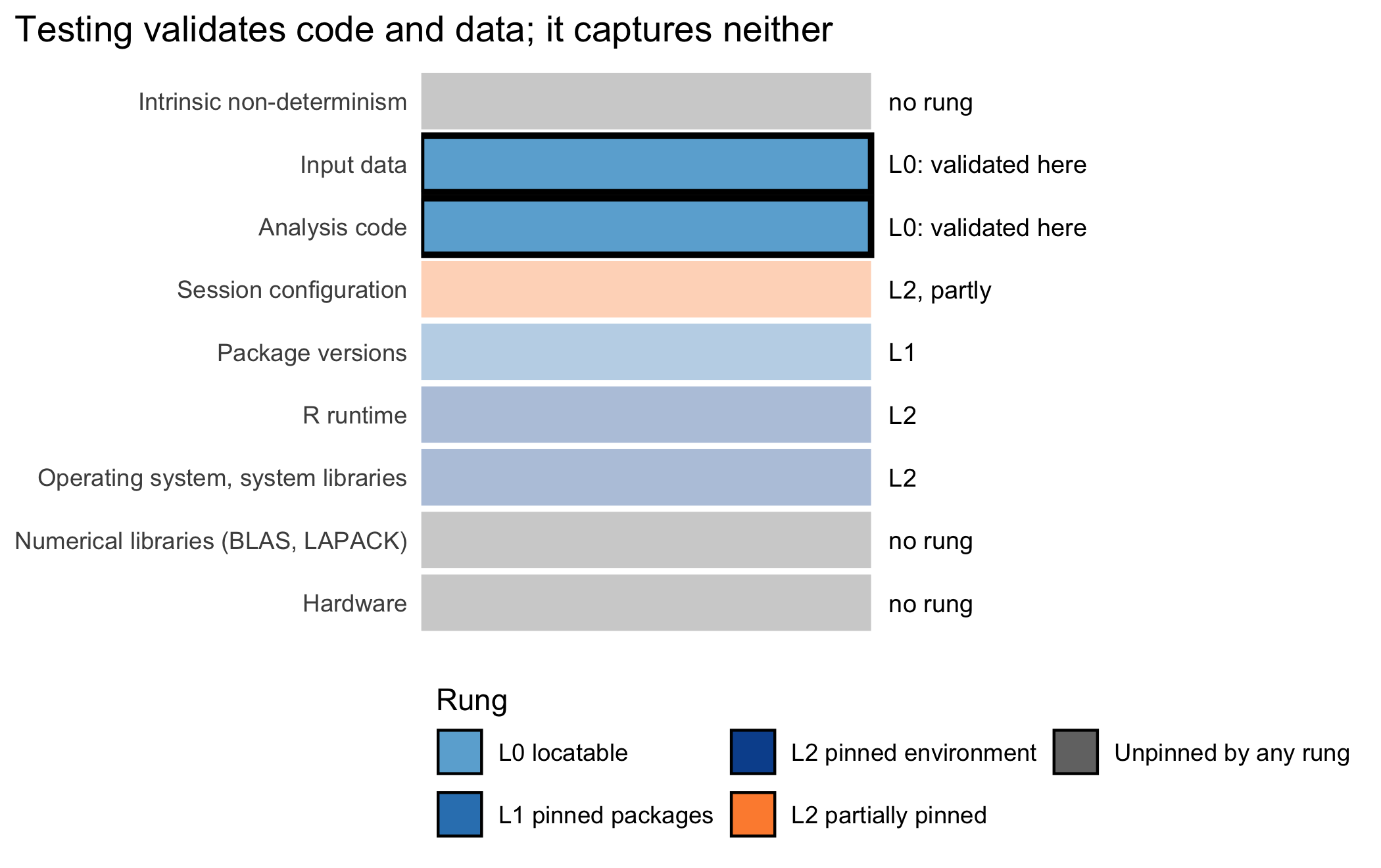
Program testing can be used to show the presence of bugs, but never to show their absence!
Edsger W. Dijkstra, Notes on Structured Programming (1972)
A function that silently sums instead of averaging will pass every rung of the reproducibility ladder and still be wrong on every machine that runs it. By the end of this chapter you will be able to say, of any computational result, whether it has merely been reproduced or actually checked. To make that distinction in your own analyses, the chapter develops the four kinds of test, among them the baseline test that Table 11.2 demonstrates on the book’s own running cohort.
Testing is this book’s clearest case of pure validation. It is also, among the chapters so far, one that captures nothing at all. That is, a test suite adds no package to the lockfile and no layer to the image. Figure 11.1 marks that asymmetry on the shared determinant stack. The two layers this chapter writes code against, the analysis code and the input data, are validated here, not captured. The surrounding chapters captured them already, and this chapter only confirms they still behave.
plot_determinant_stack(
validates = c('Analysis code', 'Input data'),
title = 'Testing validates code and data; it captures neither')Consider a registry study in which an analyst has written a small function to compute a mean biomarker value for each treatment arm. The function carries a simple bug: it sums the values but forgets to divide by their count. The analysis runs without error. It produces a table, a figure, a p-value. Sent to a colleague, cloned onto a second machine, restored from a lockfile inside a pinned container, it runs again and produces the identical table, the identical figure, the identical p-value. Every rung of the ladder of Chapter 3 is satisfied: the source is locatable, the packages are pinned, the environment is pinned. The result is perfectly reproducible, and it is wrong.
This is the reproducibility paradox, and it is the pivot of this chapter. A buggy function that returns the wrong answer returns the same wrong answer everywhere, on every machine, at every later date. Reproducibility machinery, faithfully applied, does not detect the error; it propagates it with mechanical fidelity. The lesson, pressed by Leek and Peng in their aptly titled note that reproducible research can still be wrong (Leek & Peng, 2015), is that reproducibility is a floor and not a ceiling. It guarantees that a result can be regenerated. It says nothing whatever about whether the result is correct.
The remedy is testing. But why does testing belong in a book about reproducibility, rather than in a separate book about software engineering? The reason is precisely the paradox. Pinning a package version, building a container, restoring a lockfile: each of these captures a determinant of the computation, and none of them examines whether the computation is right. Testing captures nothing. A test adds no package to the lockfile and no library to the image. What a test does is confirm that a function, a pipeline, or a dataset behaves as the analyst intended. It belongs, in the vocabulary this book has used since Chapter 1, to the validation register rather than the capture register, alongside the continuous integration and output verification of Chapter 12. Capture fixes the inputs; validation checks that the fixed inputs still produce the answer they are supposed to. A reproducible analysis without tests is trusted; a reproducible analysis with tests is checked.
There is a further and more constructive link to the ladder. The highest rung, L3 verified, is reached not by capturing more but by confirming that a recorded computational output regenerates. That confirmation is itself a test, of a particular kind we shall meet below as the baseline test, so the topmost level is defined by a test.
Testing tooling runs the checks, tallies the passes and failures, and reports them. It does not originate any of the judgments that give a test its value. Three of them underlie everything that follows.
The analyst decides what ‘correct’ means. A test compares a computed value against an expected one, and the expected one has to come from somewhere outside the code under test. This source of independent truth is called an oracle. Examples are a mean of one, two, and three that the analyst knows to be two; a count of rows that a data dictionary fixes at some known number; a coefficient that a textbook formula supplies. No tool knows the right answer. The analyst supplies it, and a test is only as trustworthy as the oracle behind it.
The analyst chooses which behaviors to pin. A function has an infinity of properties, most of them incidental to its purpose. The analyst decides which few constitute the function’s contract, the behaviors a future change must not break, and writes tests for those. This is the distinction, developed below, between testing behavior and testing implementation.
The analyst encodes the domain constraints. Consider the rules that an age lies between zero and one hundred and twenty, that a treatment arm is one of a fixed set of labels, and that a probability sits in the unit interval. These are not facts the computer can infer. They are clinical and scientific knowledge. A data-validation test is the place where that knowledge is written down in executable form, so that a violation halts the analysis rather than passing silently into a result.
tinytest. A lightweight, zero-dependency R testing framework in which a test file is a plain script of bare, top-level expectation calls (Loo, 2020).expect_equal(actual, expected), that passes or fails.lintr, without running the code.styler.A computational result depends on the code, the data, and the stack of determinants beneath them that Chapter 3 enumerated. The capture tools of Part II fix those determinants, so that the mapping from input to output is held constant across machines and across time. But holding a mapping constant says nothing about whether the mapping is the intended one. If the code encodes the function ‘sum’ where the analyst meant the function ‘mean’, then capture faithfully preserves ‘sum’, and every reproduction returns the sum. The error is not in the reproduction; the reproduction is flawless. The error is in the mapping, and the only instrument that examines the mapping is a test.
Two consequences follow, and they cut in opposite directions. On the one hand, a result that fails to reproduce is thereby shown to be untrustworthy, which is a genuine service; irreproducibility is a detectable defect. On the other hand, a result that does reproduce has been shown only to be stable, not to be right. Stability is easily mistaken for correctness by an analyst who has watched the same number appear three times. Testing exists to break the false inference from ‘it came out the same’ to ‘it came out correct’.
This chapter’s own practice reaches a baseline test on one bootstrap bound (Table 11.2) and a short, illustrative suite of unit, integration, and data-validation checks on hand-picked examples. It establishes that those particular results regenerate and that those particular functions behave as intended. It says nothing whatsoever about any function, dataset, or computation this chapter did not choose to test.
The oracle introduced above sits at the level of a single function: a hand-computed mean, a row count a data dictionary fixes. The same structure scales up to the level of the whole analysis’s primary result, and doing so closes a gap the paradox otherwise leaves open.
A pre-specified analysis plan states in advance the primary endpoint, the model, the covariates, and the comparison that will answer the study’s main question. It is also called a statistical analysis plan, or, when it is registered publicly before the data are seen, a pre-registration. Written and dated before the analyst has looked at the outcome data, it is computed independently of any code’s output in exactly the sense the Vocabulary box above requires of an oracle. That is, it specifies what the correct analysis looks like, not by running anything, but by committing in writing to a choice that the data cannot later be allowed to revise.
A function-level oracle, such as the hand-computed mean described above, catches a coding error: the function returns the wrong number for a known input. It says nothing about whether the analysis itself asks the right question. Consider an analysis built by trying several models, several covariate sets, or several endpoints and reporting the one that reached significance. It can be bug-free in every function and pass every unit test. It can also still reproduce exactly on a second machine, because reproduction only checks that the same code returns the same output. The reproducibility paradox stated above applies again, one level up. A fully reproducible analysis can still be the wrong analysis, chosen with the benefit of having already seen the answer. A pre-specified plan is the oracle that guards against this failure, because it fixes the intended analysis before the data could have shaped it.
The two oracles differ in what independence they supply. A function’s oracle is independent of the code that computes the value; a pre-specified plan is independent of the data that will later be analyzed. Both are necessary, and neither substitutes for the other. A bug-free implementation of an unregistered, data-driven analysis is still untrustworthy in the way the plan would have prevented. Conversely, a faithful implementation of a pre-specified plan can still contain a coding error that only a function-level oracle would catch.
In a research compendium, a pre-specified plan is a dated document, committed to the repository (or deposited externally, as on the Open Science Framework) before the raw data arrive, or before they are unblinded. Checking an analysis against it is not an expect_equal() call but a review step: do the fitted model’s formula, the stated primary comparison, and the decision rule actually implemented match what the plan specified? Where the match can be stated mechanically, for example that fit_model() fits the formula the plan names, a test can assert it directly. Such a test compares the model’s formula (as text, or as a parsed call) against a string recorded from the plan rather than against anything the analysis itself computed.
The framework this book uses adopts tinytest (Loo, 2020) as its testing tool. The choice rewards a moment’s explanation because it shapes how the tests look. tinytest is lightweight and carries no dependencies of its own, which matters in a reproducible compendium. Every additional test dependency enlarges the lockfile and the container image, and a testing framework that dragged in a dozen packages would tax the very machinery it is meant to protect. The more visible consequence is stylistic. A tinytest test file is an ordinary R script containing bare, top-level expectation calls, with no wrapping function around them.
A reader who has met testthat will notice the difference at once. Where testthat nests each assertion inside a test_that('description', { ... }) block, tinytest writes the assertion directly:
Each line is a complete test. The file is also a runnable script, so during development an analyst can source it directly and watch the expectations evaluate. The available expectations cover the common cases (expect_equal(), expect_true(), expect_false(), expect_identical(), expect_error(), expect_inherits(), and a few others). A compendium’s tests are collected in inst/tinytest/ and driven by a small tests/tinytest.R runner that R CMD check invokes. tinytest runs each file with the test directory as its working directory. A test that reads a project file from the root therefore reaches it through ../../, as the listings below do. We follow the convention throughout: bare top-level expectations, one concern per file, named test-<thing>.R.
A research compendium wants four kinds of test, and they form a progression from the smallest unit of code to the reproduction of a whole result. We take them in turn, illustrating each on synthetic data of the sort a health study might produce.
A unit test checks that one function behaves as intended on inputs whose correct outputs are known independently. The mean function of the orientation, here called calculate_mean, is the canonical case. Its contract is that it returns the arithmetic mean, and the oracle is arithmetic done by hand:
The first two lines pin the ordinary behavior against hand-computed answers. The third and fourth pin the edge cases, the empty vector and the missing value, which are exactly the inputs on which an untested function tends to misbehave. A unit test suite is, in effect, a written record of what the analyst believes each function promises.
A unit test exercises a function in isolation, but a health analysis is rarely one function. It is a pipeline, in which raw data is loaded, cleaned, modeled, and summarized, and the components can be individually correct yet compose incorrectly. An integration test runs the pipeline end to end and checks the result:
# abridged from inst/tinytest/test-cohort.R
raw <- load_cohort('../../analysis/data/raw_data/cohort_raw.csv')
cohort <- clean_cohort(raw)
fit <- fit_model(cohort)
summary_tbl <- summarise_fit(fit)

expect_true(is.numeric(coef(fit)))
expect_true(all(c('term', 'estimate') %in%
                names(summary_tbl)))
expect_equal(nrow(summary_tbl), 3L)
The first expectation tests the contract that coef(fit) returns numeric coefficients, which is what summarise_fit() needs to proceed. Testing expect_inherits(fit, 'lm') would also pass here, because glm inherits from lm, but it would break the moment the function was upgraded to fit_cox() returning a coxph, which does not. Testing the interface (‘does coef() return numeric values?’) survives that migration; testing the class does not. The book’s own compendium does not perform this migration: fit_cox() was added beside fit_model() rather than replacing it, and its tests sit in a file of their own, inst/tinytest/test-fit-cox.R.
The integration test does not re-check what the unit tests already cover. Instead it checks the seams: that the output of clean_cohort is a valid input to fit_model, and that the model summary has the expected shape. A pipeline that passes its unit tests can still fail here, if a column is renamed in one step and read under its old name in the next.
The third kind of test turns its attention from the code to the data. Much of what goes wrong in a health analysis is not a coding error but a data defect. Examples are an age of two hundred, a negative laboratory value, a treatment label misspelled, or a column silently dropped by an upstream export. A data-validation test encodes the analyst’s domain knowledge as executable constraints and fails when the data violates them.
Before writing constraints, we look first at what we are constraining. Table 11.1 tabulates the retinopathy trial introduced in the conventions. It is included here for a reason beyond illustration: every cell in it can be counted by hand from the data, which is precisely the property an oracle needs. A test asserting that the untreated arm contains 197 eyes, written as that literal number, is checkable by someone who does not trust the function that produced it. A test asserting that it contains nrow(subset(d, trt == 0)) eyes is not a test at all; it is the function agreeing with itself.
library(tibble)
library(knitr)

d <- survival::diabetic
d$arm <- factor(d$trt, levels = c(0, 1),
                labels = c('Untreated', 'Laser'))

arms <- tibble(
  Arm = levels(d$arm),
  Eyes = as.integer(table(d$arm)),
  Events = as.integer(tapply(d$status, d$arm, sum)),
  `Event rate` = sprintf(
    '%.3f', as.numeric(tapply(d$status, d$arm, mean))
  )
)

kable(arms, align = 'lrrr')survival::diabetic), the real dataset this book computes on. Each count is verifiable by hand from the 394 records, which is what makes the table usable as a test oracle rather than merely as a description.
| Arm | Eyes | Events | Event rate |
|---|---|---|---|
| Untreated | 197 | 101 | 0.513 |
| Laser | 197 | 54 | 0.274 |
The difference between the arms is large and in the expected direction. That is a reason to be careful rather than pleased, because a validation test should assert what the protocol requires, not what this particular extract happens to show. An assertion that the event rate in the laser arm is below one third would pass today. It would fail on a different trial, or on a corrected export, for reasons having nothing to do with a defect.
# abridged from inst/tinytest/test-cohort.R
raw <- load_cohort('../../analysis/data/raw_data/cohort_raw.csv')
cohort <- clean_cohort(raw)

# the expected columns are present
expect_true(all(c('mrn', 'age_at_enroll', 'sex', 'incident_dm')
                %in% names(raw)))

# ages lie within the enrollment criteria, not merely
# within the observed range
expect_true(all(cohort$age_at_enroll >= 18 &
                cohort$age_at_enroll <= 105, na.rm = TRUE))

# sex takes only its two coded levels once cleaned
expect_true(all(cohort$sex %in% c('F', 'M')))

# outcome missingness stays within what the analysis
# can tolerate
expect_true(mean(is.na(cohort$incident_dm)) < 0.15)
These are the tests that most directly repay a health scientist, because they catch the errors that no amount of correct code can prevent, the errors that live in the data before the analysis begins. In a data-analysis or simulation archetype, where there may be few reusable functions to unit-test, the data-validation tests often carry most of the suite’s weight.
The fourth kind closes the loop back to the ladder. A reproducibility test checks that a recorded result regenerates. Its most tempting form runs a seeded procedure twice in one session and asserts that the two results agree:
# a same-session check: it cannot detect what it
# appears to guard against
expect_equal(bootstrap_ci(cohort, B = 2000, seed = 2024),
             bootstrap_ci(cohort, B = 2000, seed = 2024))
Note first where the seed lives. bootstrap_ci() takes it as an argument and sets it internally, with withr::with_seed(), which also restores the caller’s generator state on exit. As a result, the function is deterministic given its arguments and does not disturb any random stream around it. A procedure that depends on the caller setting a seed first is one set.seed away from irreproducible, and moving the seed into the signature makes forgetting it impossible.
A same-session check cannot fail for the reason it seems to serve. Both calls run in the same R, under the same random-number defaults, with the same package versions. When an upgrade changes how sample() draws, as R 3.6.0 did, both calls change together and still agree. What the check does catch is narrower: a procedure that ignores its seed. That is worth one line in a unit test, but it is not a reproducibility test.
A reproducibility test that can fail compares today’s result with one recorded in an earlier session and committed to the repository. We call it a baseline test. It has three parts: a script, run once, that records the baseline; the committed baseline file; and a test file that recomputes the quantities and compares them with a stated tolerance.
# analysis/scripts/generate_baseline.R, abridged. Run once
# from the project root to record the baseline, then commit
# inst/baseline/cohort_baseline.rds.
# The book's own baseline was recorded this way, and the
# file is now committed at that path; regenerate it only
# if the generator, the seed, or the model change.
result <- run_canonical_analysis(
  'analysis/data/raw_data/cohort_raw.csv'
)
dir.create('inst/baseline', recursive = TRUE,
           showWarnings = FALSE)
saveRDS(result, 'inst/baseline/cohort_baseline.rds')
# inst/tinytest/test-baseline-cohort.R, abridged: the
# real file also searches fallback paths for both files
raw_path <- '../../analysis/data/raw_data/cohort_raw.csv'
if (!file.exists(raw_path)) {
exit_file('raw extract absent; run simulate_cohort.R')
}
baseline <- readRDS(
system.file('baseline', 'cohort_baseline.rds',
package = 'reproducibility'))
result <- run_canonical_analysis(raw_path)
expect_equal(result$n_rows, baseline$n_rows,
info = 'cleaned row count matches baseline')
expect_equal(result$n_events, baseline$n_events,
info = 'event count matches baseline')
expect_equal(result$hr, baseline$hr, tolerance = 1e-8,
info = 'Cox HR matches committed baseline')
expect_equal(result$lower, baseline$lower,
tolerance = 1e-8,
info = 'lower CI bound matches committed baseline')
expect_equal(result$upper, baseline$upper,
tolerance = 1e-8,
info = 'upper CI bound matches committed baseline')Three details carry the weight. The path is relative to inst/tinytest/, where tinytest runs the file. The guard lets the file exit early under R CMD check, which installs the package without analysis/. The mirror in inst/testdata/ covers the unit and data-validation tests; the baseline test requires the raw extract and skips cleanly without it. Finally, the tolerance is stated and chosen, not left at a default. 1e-8 relative is wide enough to absorb floating-point summation reordered by a different BLAS or thread count (Chapter 7), and far too narrow for a change in the fitted coefficients to pass. A comparison with no tolerance would fail on that reordering, and a check that fails for reasons unrelated to the analysis trains its reader to ignore it.
The test can be watched failing for the reason it exists. The chunk below plays both sessions on the synthetic cohort. It records the 97.5 percent bootstrap bound for mean BMI under the sampler R used before version 3.6.0 (sample.kind = 'Rounding'), as an analysis recorded on an older R would have. It then reruns it with the same seed and sampler, and reruns it again with the same seed under the current default ('Rejection'). The comparison is the one expect_equal() makes, all.equal() at the stated tolerance. withr::with_seed() sets the sampler only for the duration of each call, and the final stopifnot() confirms the session’s generator is as it was.
library(knitr)

cohort <- read.csv('../data/raw_data/cohort_raw.csv')
bmi <- cohort$bmi[!is.na(cohort$bmi)]

boot_upper <- function(x, seed, sample_kind, reps = 2000) {
  withr::with_seed(
    seed,
    {
      means <- replicate(reps, mean(sample(x, replace = TRUE)))
      unname(quantile(means, 0.975))
    },
    .rng_sample_kind = sample_kind
  )
}

kind_before <- RNGkind()[3]

# R warns whenever the pre-3.6.0 sampler is selected;
# the warning is expected here and muffled.
baseline <- suppressWarnings(boot_upper(bmi, 2024, 'Rounding'))
rerun_same <- suppressWarnings(boot_upper(bmi, 2024, 'Rounding'))
rerun_new <- boot_upper(bmi, 2024, 'Rejection')

tol <- 1e-8
passes <- function(current) {
  isTRUE(all.equal(current, baseline, tolerance = tol))
}

checks <- data.frame(
  run = c('recorded baseline (Rounding)',
          'rerun, same seed and sampler (Rounding)',
          'rerun, same seed, current default (Rejection)'),
  upper_bound = c(baseline, rerun_same, rerun_new),
  passes = c('(baseline)',
             ifelse(passes(rerun_same), 'yes', 'no'),
             ifelse(passes(rerun_new), 'yes', 'no'))
)

stopifnot(identical(RNGkind()[3], kind_before))

kable(checks, digits = 4,
      col.names = c('Run', '97.5% bootstrap bound',
'Passes at tolerance 1e-8'))| Run | 97.5% bootstrap bound | Passes at tolerance 1e-8 |
|---|---|---|
| recorded baseline (Rounding) | 29.1400 | (baseline) |
| rerun, same seed and sampler (Rounding) | 29.1400 | yes |
| rerun, same seed, current default (Rejection) | 29.1436 | no |
The rerun under the current sampler moves the bound by 0.0036 units of BMI, from 29.1400 to 29.1436. That is a small number, and it is not a numerical artifact: the resamples themselves are different. The baseline test reports it; two calls in one session, both under whichever sampler the session uses, would have agreed with each other and reported nothing.
Failing the seed-exact comparison is not the same as failing to reproduce the result, because the bound is itself a Monte Carlo estimate. The chunk below estimates its Monte Carlo standard error (MCSE) as the standard deviation of the bound over 40 seeds, at the table’s 2000 replicates, and then applies a two-tier check to the two reruns.
mc_bounds <- vapply(1:40, function(s) boot_upper(bmi, s, 'Rejection'),
                    numeric(1))
mcse <- sd(mc_bounds)
two_tier <- compare_to_baseline(c(rerun_same, rerun_new),
                                c(baseline, baseline), mcse = mcse)
two_tier
#> [1] "exact"                    "within Monte Carlo error"

# Decimals an MCSE supports: the MCSE must be below half a
# unit of the last reported digit.
digits_supported <- function(mcse) max(0, floor(-log10(2 * mcse)))
d_bmi <- digits_supported(mcse)
# An MCSE from 40 seeds is itself uncertain by about 11
# percent, so two significant figures are all it supports.
sig2 <- function(x) {
  formatC(signif(x, 2), digits = 2, format = 'fg', flag = '#')
}
stopifnot(round(baseline, d_bmi) == round(rerun_new, d_bmi))
The MCSE of the bound is 0.015, so the sampler change is about 0.2 of one MCSE. The seed-exact comparison fails, yet the change is a fraction of one MCSE, and the statistical result reproduces.
This is the two-tier baseline check. The first tier compares at the numerical tolerance 1e-8; a pass means the draws themselves regenerated. On a failure, the second tier accepts a difference of at most three MCSE, with the MCSE recorded beside the baseline value. compare_to_baseline() in the book’s package implements both tiers, and it returns ‘exact’ for the same-sampler rerun and ‘within Monte Carlo error’ for the current sampler. Both the recorded value and the rerun carry Monte Carlo error, so their difference has a standard deviation of about \(\sqrt{2}\) MCSE. Under normality, three MCSE then flags a pure change of draws about 3.4 percent of the time, which is the price of a second tier that still catches a real change.
The second tier applies only to a quantity that has Monte Carlo error, such as a bootstrap bound or a simulation summary. The Cox hazard ratio and its confidence limits in test-baseline-cohort.R are deterministic functions of the data, so only the first tier applies to them, and compare_to_baseline() with mcse = NULL reduces to it. The precision of the table follows the same distinction. Its four decimals are there for the seed-exact tier. As a statistical result, an MCSE of 0.015 supports reporting the bound as 29.1 under either sampler, by the rule the next section gives.
A baseline test is what L3 requires. The top rung, as Chapter 3 defines it, asks that recorded outputs be shown to regenerate within a stated tolerance from a clean rebuild. The baseline test supplies the recorded outputs and the tolerance; running it inside an environment rebuilt from its recipe supplies the clean rebuild, and Chapter 12 assembles the two in continuous integration. A suite with no baseline test can show that the code runs and that its functions are correct on known inputs. However, it cannot show that a recorded result regenerates, so it does not reach L3 however thorough it is. In the zzcollab composition, zzc verify --full applies this rule. It stamps L3 only when the image rebuilds, the test suite passes, and at least one inst/tinytest/test-baseline*.R file exists and is named in the test log. Otherwise it reports the project as rebuilt and tested, at L2, with no baseline comparison. A baseline whose guard exits early is still named in the log, so the guard must not fire in the image.
Table 11.2 fixed the seed and varied only the sampler (the default that R changed in version 3.6.0), which isolated one source of change in the bootstrap bound. A second source is always present and has nothing to do with R versions. A bootstrap estimate is itself a Monte Carlo quantity, built from a finite number of resamples. It carries its own sampling variability on top of the statistical sampling variability of the original cohort. Two bootstrap runs at different seeds, same data, same number of replicates B, will not return exactly the same bound. The standard deviation of the bound across seeds is its Monte Carlo standard error (MCSE), distinct from the standard error the bootstrap is estimating.
But how much does such a bound move in practice? The practical diagnostic needs no extra theory: rerun the same call at many seeds for a given B, and take the standard deviation of the result; then raise B and watch it shrink. The chunk below does this with bootstrap_ci() on the HbA1c odds ratio, at B = 250 and at the package default B = 1000, with 20 seeds each.
cohort <- clean_cohort(
  load_cohort('../../analysis/data/raw_data/cohort_raw.csv')
)
bounds_at <- function(B) {
  t(vapply(1:20, function(s) bootstrap_ci(cohort, B = B, seed = s),
           numeric(2)))
}
b250 <- bounds_at(250)
b1000 <- bounds_at(1000)
mcse250 <- apply(b250, 2, sd)
mcse1000 <- apply(b1000, 2, sd)
ratio <- mcse250 / mcse1000
# With 20 seeds the log of a ratio of two SDs has a standard
# error near sqrt(2 / 38); the prose calls the ratios
# consistent with 2 only while they are within two of them.
stopifnot(all(abs(log(ratio / 2)) < 2 * sqrt(2 / 38)))
d_upper <- digits_supported(mcse1000['upper'])
d_lower <- digits_supported(mcse1000['lower'])
stopifnot(d_upper < 2)
ci_default <- bootstrap_ci(cohort)
# Replicates for the MCSE to fall below half a unit of one
# more decimal, scaling the observed MCSE by 1/sqrt(B).
B_for <- function(mcse, d, B = 1000) {
  ceiling(B * (mcse / (0.5 * 10^-d))^2)
}
B_upper_next <- B_for(mcse1000['upper'], d_upper + 1)
At B = 250 the MCSE of the upper bound is 0.43 and that of the lower bound is 0.072. At B = 1000 they are 0.22 and 0.040, on bounds near 5.5 and 1.5. An MCSE that scales as \(1/\sqrt{B}\) halves when B is quadrupled, and the observed ratios are 2.0 for the upper bound and 1.8 for the lower. With 20 seeds, each estimated standard deviation is itself uncertain by about 16 percent, so these ratios are consistent with that scaling but do not pin it closely.
The standard guidance for simulation studies is to report the MCSE of every Monte Carlo estimate and to choose the number of repetitions from the precision required (Morris et al., 2019). Applied to reported digits, it gives a rule for the number of replicates. Choose B so that the MCSE of each reported quantity is below about half a unit of its last reported digit, or report only the digits the MCSE supports. At the default B = 1000 the rule allows the lower bound 1 decimal place and the upper bound 0, so the default call’s interval should be reported as 1.5 to 5. Reporting the upper bound to one more decimal would need about 19,000 replicates. A two-decimal interval from bootstrap_ci() at its default therefore prints digits that are Monte Carlo noise. The baseline test’s 1e-8 in Table 11.2 is a numerical tolerance for one fixed sequence of draws, and it says nothing about this. The MCSE is estimated once, when choosing B, and recorded with the baseline as the scale of the second tier; the test suite does not re-estimate it on every run.
Resampling at the B a real analysis needs is often parallelized across cores, and the random streams then need as much care as the seed. Naive parallelization fails first by irreproducibility. Under the default Mersenne-Twister generator and the default mc.set.seed = TRUE, parallel::mclapply() discards the inherited generator state in each child process, which then seeds itself from the clock and its process id. A set.seed() before the call therefore does not fix the result, and two runs differ. With mc.set.seed = FALSE the children inherit the parent’s state, and the workers draw identical streams, so supposedly independent replicates are duplicated. The L’Ecuyer-CMRG generator, which RNGkind('L\'Ecuyer-CMRG') selects, was built to provide many independent streams. Under it, mclapply() gives each child its own stream, and parallel::clusterSetRNGStream() gives one to each worker of a cluster. Per-worker streams are independent, but the result still depends on the number of workers. The replicates are divided among the workers in chunks, so a given replicate draws from a different stream when the worker count changes.
Invariance to the worker count needs per-task streams: one stream for each replicate, fixed before any worker starts. parallel::nextRNGStream() can precompute them, the future.apply package does so with future.seed = TRUE, and the doRNG package does so for a foreach loop. The book’s package provides replicate_streams(), which precomputes the streams with nextRNGStream() and runs the replicates with mclapply(). The chunk below runs the same 2000 bootstrap means of BMI on one worker and on two. Forking is unavailable on Windows, where both runs are sequential and the comparison is trivially true.
The two runs are identical (TRUE), replicate by replicate, because replicate i draws from stream i wherever it runs. The same seed discipline that makes a serial bootstrap reproducible extends to a parallel one only in this per-task form.
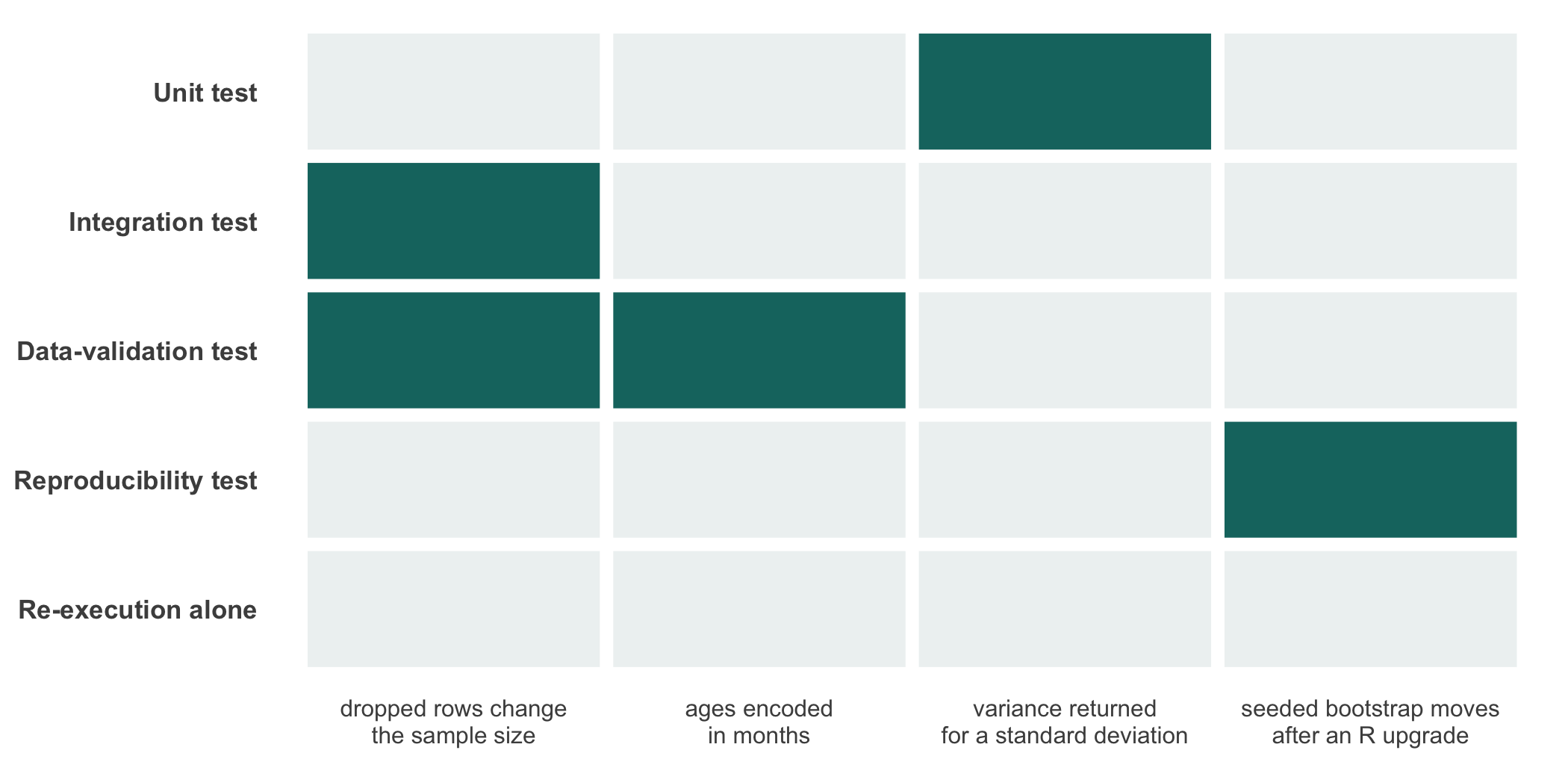
Each of the four kinds catches defects the others do not see, and Figure 11.2 sets four representative defects against them. Start with the bottom row. Re-execution alone, with no test of any kind, catches none of the four, because every one of these defects is deterministic and will reproduce perfectly. That row is the reproducibility paradox in tabular form.
library(ggplot2)
library(tibble)

defects <- c('dropped rows change\nthe sample size',
             'ages encoded\nin months',
             'variance returned\nfor a standard deviation',
             'seeded bootstrap moves\nafter an R upgrade')
kinds <- c('Re-execution alone',
           'Reproducibility test',
           'Data-validation test',
           'Integration test',
           'Unit test')

cover <- expand.grid(defect = defects, kind = kinds,
                     stringsAsFactors = FALSE)
cover$defect <- factor(cover$defect, levels = defects)
cover$kind <- factor(cover$kind, levels = kinds)

hits <- c('Unit test|variance returned\nfor a standard deviation',
          'Integration test|dropped rows change\nthe sample size',
          'Data-validation test|dropped rows change\nthe sample size',
          'Data-validation test|ages encoded\nin months',
          'Reproducibility test|seeded bootstrap moves\nafter an R upgrade')
cover$catches <- paste(cover$kind, cover$defect, sep = '|') %in% hits

ggplot(cover, aes(x = defect, y = kind)) +
  geom_tile(aes(fill = catches), color = 'white', linewidth = 2) +
  scale_fill_manual(values = c('TRUE' = '#14746f',
                               'FALSE' = '#eef2f2'),
                    guide = 'none') +
  labs(x = NULL, y = NULL) +
  theme_minimal(base_size = 9) +
  theme(
    panel.grid = element_blank(),
    axis.text.x = element_text(size = 7.6, lineheight = 0.95),
    axis.text.y = element_text(face = 'bold', size = 8.4)
  )
A test is worth writing only if it survives changes that ought not to break it and fails on changes that ought to. The way to secure this is to test what a function does, its observable behavior, rather than how it does it, its internal implementation. The distinction is easiest to see in a pair of tests for the same function:
The first test asserts that my_clean uses a function called filter internally. If the analyst later rewrites my_clean in base R, removing the filter call while leaving its behavior unchanged, the first test fails. It fails for no good reason: the function still does exactly what it promised. Such a test punishes honest refactoring and trains the analyst to distrust the suite. The second test asserts only that the cleaned data carries no missing values, which is the behavior that actually matters. It passes under any correct implementation. As a general rule, a test should fail when, and only when, the function’s contract is broken. Tests that fail for other reasons are a tax on maintenance. Wilson and colleagues, in their best-practices and good-enough-practices guidance, make behavioral testing a recurring recommendation (Wilson et al., 2014; Wilson et al., 2017).
A corollary concerns how much to test. A test that merely confirms a result is a data frame, without checking any value in it, tests too little and gives false comfort. A test that pins every incidental property tests too much and breaks on every revision. Deciding what to pin is the second of the analyst’s contributions named above, and no tool makes that decision.
Testing confirms that code is correct. A second family of tools confirms that code is legible and consistent. Although these tools do not check correctness directly, they belong to the same validation register and serve the same reproducibility end. The argument is one of mechanism. Code that a reader can follow is code whose errors a reader can find. Consistent formatting removes the visual noise that hides a transposed argument or a misplaced parenthesis. Moreover, a single house style across a compendium means that a difference in the code is always a difference in meaning, never merely a difference in whitespace. Wilson and colleagues, in both of their practice papers, treat readable, conventional code as a component of reproducible work rather than an aesthetic preference (Wilson et al., 2014; Wilson et al., 2017). Sandve and colleagues, in their ten simple rules, make the companion point that the provenance and the recorded results of an analysis must themselves be preserved (Sandve et al., 2013).
Two tools mechanize this, and a third enforces them.
Linting is static analysis: lintr reads the source without running it and flags stylistic deviations and likely errors. Examples are an assignment with = where the house style is <-, a line past the width limit, a variable assigned and never used, and a call to a function that does not exist. Because it does not execute the code, it catches a class of mistake that tests, which only exercise the paths they call, may miss.
Styling is automatic reformatting: styler rewrites the source into a consistent layout, fixing indentation, spacing, and alignment, so that formatting is never a matter for human attention or for a code review. The two are complementary; styler fixes the formatting that lintr would otherwise complain about.
In the framework, both run inside the project container through Makefile targets, so that no host R installation is required and every collaborator runs the identical checks:
$ make style   # reformat R code with styler
$ make lint    # analyze R code with lintr
A pre-commit hook enforces them. A hook is a script that git runs automatically at a defined moment; a pre-commit hook runs before a commit is recorded, and can refuse the commit if a check fails. Configuring the linter and styler as a pre-commit hook means that unstyled or unlinted code cannot be committed from a clone where the hook is installed, unless the analyst bypasses it with git commit --no-verify. That is a stronger guarantee than a convention that relies on memory, but a clone does not carry the hook with it. The configuration lives in a .pre-commit-config.yaml file at the project root:
# .pre-commit-config.yaml
repos:
  - repo: https://github.com/lorenzwalthert/precommit
    rev: v0.4.3
    hooks:
      - id: style-files
      - id: lintr
      - id: readme-rmd-rendered
      - id: no-browser-statement
With this in place, an attempt to commit code that styler would reformat, or that lintr flags, or that contains a stray browser() left over from debugging, is stopped before the commit completes. The analyst is then prompted to fix it. The hook is the fast local gate. A collaborator who has not installed it is caught only if continuous integration (Chapter 12) runs the same checks on the server. The workflows in that chapter do not, so a project that relies on the hook should add a step running lintr::lint_dir() there.
Every use of ‘validation’ in this chapter has been the statistical and software-engineering sense: checking that code is correct, that data meet a constraint, that a result regenerates. In pharmaceutical, medical-device, and other FDA- or EMA-regulated work, ‘validation’ names a broader and more procedural idea. Chapter 3’s warning box introduces the distinction; this section develops the three practices that fill it out for testing specifically.
Computer system validation. Under 21 CFR 11.10(a), a closed system that creates, modifies, maintains, or transmits regulated electronic records must be validated ‘to ensure accuracy, reliability, consistent intended performance, and the ability to discern invalid or altered records’ (21 CFR Part 11, n.d.). The European Medicines Agency sets parallel expectations for computerized systems in clinical trials, and names statistical software among them (European Medicines Agency, GCP Inspectors Working Group, 2023). This is validation of the system across its lifecycle, documented once and maintained by a change-control process, not a one-time test run. The regulation does not say how that validation is shown. Installation, operational, and performance qualification (IQ, OQ, and PQ) come from qualification practice, in which a system qualification typically executes all three (Nicholls et al., 2020), not from the text of 11.10. The requirement’s reach is also narrower than its wording suggests. FDA’s 2003 guidance on the scope and application of Part 11 states that the agency will exercise enforcement discretion over the Part 11 validation requirement, while the predicate rules, the underlying requirements of the Act and of FDA’s other regulations, still apply, their own validation requirements included (U.S. Food and Drug Administration, 2003). The R Validation Hub concludes that Part 11 is not relevant or mandatory for statistical analysis software itself, though elements of it apply when R is used as part of a validated system (Nicholls et al., 2020). What an inspector asks in practice is whether the statistical computing environment is in a documented, validated state under the sponsor’s standard operating procedures and the predicate rules. A tinytest suite that passes is evidence toward that state. It is not, by itself, that state, which also rests on qualification records and a record of who approved each change and when.
Double programming. Independent of any code-based test, a regulated submission is commonly checked by double programming. Two analysts, or one analyst and an independent reviewer, implement the same analysis separately, from the same specification, usually in isolation from each other’s code. The two results are then compared. This is a different reproducibility practice from everything else in this chapter. A baseline test reruns the same code and checks that it still returns the same answer; double programming runs two different implementations of the same specification and checks that they agree. Consider a bug shared by both implementations, because both analysts misread the same ambiguous protocol sentence. It would pass a baseline test (the code is unchanged) and would also pass double programming (the two analysts made the same mistake). What double programming catches is a bug particular to one implementation, the error a single analyst’s code review is least likely to find in their own work.
Package risk assessment. Pinning package versions, as Chapter 6 teaches, fixes which code runs. It says nothing about how much to trust that code. But how is that trust to be judged? The R Validation Hub, an R Consortium working group formed for exactly this question, proposes a risk-based answer (Nicholls et al., 2020). The first step is to classify each package as either ‘intended for use’ (called directly by the analysis) or an unexamined dependency reached only through another package. The second is, for each intended-for-use package, to assess its purpose, maintenance practice, community usage, and existing test coverage. The third is to have a qualified reviewer record a documented risk judgment. Higher risk earns additional targeted testing. Base R and the recommended packages are treated as minimal risk. For other widely used packages, such as the tidyverse, the white paper says only that there is a reasonable case to treat their maintainers as a trusted resource, and leaves that decision to each organization. Whatever the risk score, tests are still required for the statistical modeling functions of an intended-for-use package. The riskmetric package operationalizes several of these metrics so the assessment does not start from nothing. This is a judgment about trustworthiness layered on top of the pinning Chapter 6 already does, not a replacement for it.
Double programming is costly, because it implements every output it covers twice. Most analyses, regulated or not, are checked instead by review: a second analyst reads a proposed change, usually as a pull request (Chapter 4), and approves it before it merges. The two practices find different errors. A reviewer reads one implementation against the plan, and is well placed to see a wrong exclusion, a covariate the plan does not name, or a seed set in the wrong place. A reviewer is poorly placed to see an arithmetic slip in code that reads correctly, which is the error a second, independent implementation exposes. The choice between them is therefore a judgment about risk, made per output and recorded. One defensible arrangement is to double-program the outputs a decision rests on, such as the primary estimate, and to review the rest.
A reviewer needs a short list rather than a general impression. For a pull request that changes an analysis, we suggest six questions.
.Rprofile or nowhere?The list draws on the book’s gates, but it is not a gate. It asks for the judgments that continuous integration cannot make (Chapter 12): whether a threshold matches the plan, and whether a changed test was changed for a good reason. The approval on the pull request then records who checked the change and when, the same kind of record the validated state described above rests on. Questions 3 and 5 take the longest, because answering them means opening the plan and the test diff rather than reading the code alone.
The four kinds of test are the same in every compendium, but their relative weight shifts with the archetype. Table 5.2 in Chapter 5 is the reference. We state the shift here so that a student who has met testing only in the context of R packages does not wrongly conclude that a data analysis has nothing to test. Testing is native to the R-package archetype, whose suite is dominated by unit tests that R CMD check runs as a matter of course. The data-analysis and simulation archetypes, by contrast, may have few reusable functions and no exported interface. In these the data-validation and reproducibility tests carry the weight instead. A simulation in particular leans on a baseline test that fixes the seed and compares the result with a committed value, since its entire output is a function of that seed. Chapter 12 develops the point at length. The manuscript archetype adds a test that the report renders and that its headline numbers match a baseline. The blog archetype tests the functions and example computations its posts depend on. That is a reproducibility obligation to readers no smaller than a manuscript’s to its reviewers.
We now make the paradox concrete and executable. The following chunk defines the calculate_mean function in two forms, one correct and one carrying the bug of the orientation, and checks each against three inputs whose means are known by hand. Rather than call the tinytest package, which may be absent from a bare R session, we hand-roll a one-line expectation. That is all a bare check really is: a comparison of an actual value against an expected one.
# the function under test, in a correct and a
# buggy form
calculate_mean <- function(x, na.rm = FALSE) {
  if (na.rm) x <- x[!is.na(x)]
  sum(x) / length(x)
}

calculate_mean_buggy <- function(x) {
  sum(x)                 # bug: division dropped
}

# a minimal hand-rolled expectation: no testing
# package required
expect <- function(actual, expected, tol = 1e-8) {
  isTRUE(abs(actual - expected) < tol)
}

# three inputs whose means are known independently
cases <- list(c(1, 2, 3),
              c(10, 20, 30, 40),
              c(5, 5, 5, 5, 5))
oracle <- c(2, 25, 5)

results <- data.frame(
  input = vapply(cases,
                 function(x) paste(x, collapse = ', '),
                 character(1)),
  expected = oracle,
  correct = vapply(cases, calculate_mean, numeric(1)),
  buggy = vapply(cases, calculate_mean_buggy,
                 numeric(1))
)
results$correct_passes <-
  mapply(expect, results$correct, oracle)
results$buggy_passes <-
  mapply(expect, results$buggy, oracle)

knitr::kable(results)| input | expected | correct | buggy | correct_passes | buggy_passes |
|---|---|---|---|---|---|
| 1, 2, 3 | 2 | 2 | 6 | TRUE | FALSE |
| 10, 20, 30, 40 | 25 | 25 | 100 | TRUE | FALSE |
| 5, 5, 5, 5, 5 | 5 | 5 | 25 | TRUE | FALSE |
The correct function passes every check; the buggy function fails every check, and it fails them identically. Were we to rerun this chunk a thousand times, on a thousand machines, the buggy column would hold the same wrong values every time. The bug is not a source of variability, which reproducibility tooling might eventually surface. It produces the same error on every run, and only a comparison against an independent oracle can catch it. That comparison is what a test is.
In a real compendium, the hand-rolled expect gives way to the tinytest expectations, and the checks live in a file under inst/tinytest/. The following is that file, shown as a static listing that is not run here. It is exactly the unit test that would have caught the bug before it reached a result:
The runner tests/tinytest.R that R CMD check invokes is a three-line file:
# tests/tinytest.R
if (requireNamespace('tinytest', quietly = TRUE)) {
  tinytest::test_package('mycompendium')
}
and the pre-commit configuration shown earlier completes the picture. The linter and styler guard the code’s legibility on every commit, and the tinytest suite guards its correctness. Continuous integration re-runs both on a clean machine, so that neither guarantee depends on the author’s local setup.
A language model is a capable assistant for writing tests, and a dangerous one for a specific reason: it can readily produce tests that pass, which is not the same as tests that are correct. The analyst’s verification duty is heaviest exactly where the model is most fluent.
One rule comes first (habit 3). Never paste or upload protected health information, identifiable records, or data held under a data use agreement, nor outputs derived from them, into a model or a coding agent unless three conditions all hold. The institution has approved that endpoint for that class of data. The IRB protocol and the consent permit the processing. The data use agreement, or the provider’s terms, permits it. If any of the three is unclear, the answer is no.
The third condition is the one most often missed. Institutional approval of a tool does not override the terms under which a data provider released the data. NIH, for example, treats sharing controlled-access data through prompts with public generative AI tools, which it glosses as third-party tools, as a breach of the data use certification. It treats a model trained on such data as a data derivative, to be shared only with other approved users and not kept after the project closes (National Institutes of Health, 2025).
Describe the structure instead: the column names and types, or a small synthetic example generated from the data dictionary, never edited from real rows. A coding agent sees whatever files are in its working tree, so run it in a checkout or container where the real data is not mounted.
An agent also acts, so confine it to a branch and keep merges, pushes, and deposits for yourself (Section 2.10.1).
Tests sit close to the data, so the derived outputs the rule covers include a failing test’s printout of offending rows. The book’s simulated cohort is a suitable synthetic example to describe instead.
Prompt. ‘Here is my calculate_mean function. Write tinytest unit tests for it, including edge cases.’
Watch for. Check whether each expected value was derived by running the function it was given, rather than by independent computation. If the function is buggy, an oracle derived that way matches the bug, producing tests that pass against wrong behavior and thereby certifying the error. Check also for tests of only the paths the code obviously takes, which miss the empty vector or the missing value.
Verification. Check every expected value by hand or from an independent formula, not by running the function, since the oracle must come from outside the code under test. Confirm that the edge cases you care about, the empty input, the single value, the missing value, each have a test.
Prompt. ‘Here is the data dictionary, not the data, for my cohort: age_at_enroll (integer, years), sex (character, coded F or M after cleaning), bmi (numeric, kg/m^2), incident_dm (integer, 0 or 1). Write tinytest data-validation tests for a data frame with these columns.’
Watch for. Check for generic checks, such as non-missing identifiers and numeric outcomes, that are reasonable but do not encode your domain. The dictionary gives types and codes. It does not give the protocol’s eligibility ages, the plausible range of BMI in your population, or how much outcome missingness the analysis can tolerate, so any such bound in the answer was supplied by the model rather than by your protocol.
Verification. Supply the domain constraints yourself, or check that the generated ranges match your data dictionary. A validation test asserting a plausible-looking but wrong range is worse than no test, because it lends false authority.
Prompt. ‘Explain why this test is failing.’
Watch for. The model may recommend changing the test to match the current output, which makes the failure disappear without establishing whether the code or the test was wrong. A failing test is sometimes correct: it may be reporting a real bug.
Verification. Decide first, from the oracle, whether the code or the expectation is at fault, and only then change the one that is wrong. Never silence a failing test by editing its expected value to whatever the code currently returns; that converts a test into a tautology.
A better prompt. ‘The attached tinytest file fails on the line shown, with this message. The expected value was computed by hand from the analysis plan. Do not edit the test file. List the possible causes in the function, and for each give an input I can run, with its hand-computed answer, that would confirm or rule it out.’
A coding agent with write access need not stop at a recommendation: asked to make the suite pass, it can make the edit itself, and the change arrives as an ordinary commit. Treat inst/tinytest/ and inst/baseline/ as protected paths, and read every line of any diff that touches them before it merges, as question 5 of Section 11.12 asks. What an agent may change and what stays with the analyst is set out in Section 2.10.1.
The chapter has introduced four kinds of test. This section applies all four to the running cohort compendium, using the canonical Cox analysis as the analysis under test.
The canonical analysis. The primary question is: does BMI predict time to incident diabetes after adjusting for age and sex? The model is a Cox proportional-hazards model fit to the cleaned extract, with BMI expressed per 5 kg/m^2 so that the hazard ratio has a clinically natural scale. The analysis runs clean only after clean_cohort() has repaired the four planted defects.
The hazard ratio for BMI per 5 kg/m^2 is 1.83 (95% CI 1.32–2.52), based on 48 events from 337 cleaned rows. Uncleaned, the analysis would still run, but it would fit a different model to the 338-row raw extract, with the duplicate and the miscoded sex included.
Unit tests of fit_cox(). A unit test checks the contract of one function in isolation. For fit_cox() the contract is about which rows the model uses. coxph() drops every row with a missing value on any variable it reads, so the model uses the complete cases on followup_days, incident_dm, bmi, age_at_enroll, and sex, and its event count is the number of events among those cases, not the number of non-missing outcomes. The oracle is computed from the data directly rather than from the fit, so a change to the exclusion rule fails the test. The assertions below are in inst/tinytest/test-fit-cox.R.
model_vars <- c('followup_days', 'incident_dm', 'bmi',
                'age_at_enroll', 'sex')
complete <- stats::complete.cases(cohort[, model_vars])

expect_equal(fit$n, sum(complete),
  info = 'the model uses the complete cases on its variables')
expect_equal(fit$nevent,
             sum(cohort$incident_dm[complete] == 1),
  info = 'the event count is the events among complete cases')
expect_true(fit$nevent < sum(!is.na(cohort$incident_dm)),
  info = 'events are fewer than non-missing outcomes')
On the cleaned cohort the model uses 305 of the 337 rows, and its 48 events are the rows among them with incident_dm equal to 1. A count of non-missing outcomes, here 305, would count the zeros as events too. The same file also removes the age of one event row and checks that exactly one event and one row leave the model.
Integration test of the pipeline. An integration test checks that the pipeline stages compose correctly end to end: load_cohort feeds clean_cohort feeds fit_cox feeds summarise_cox, and the final result is a list with the expected names and no NA values. This listing and the two after it are illustrative and abridged, and the book’s suite does not run them as written.
Data-validation tests. The planted pathologies give the data-validation suite something real to catch. The test file checks each defect before and after cleaning, so a change to clean_cohort() that accidentally fixes or breaks a defect fails a test instead of silently altering the baseline.
# Duplicate before cleaning, gone after
expect_equal(sum(duplicated(raw$mrn)), 1,
  info = 'raw extract has exactly one duplicated MRN')
expect_equal(sum(duplicated(cohort$mrn)), 0,
  info = 'cleaned cohort has no duplicated MRN')

# Implausible age before cleaning
expect_true(any(raw$age_at_enroll > 105, na.rm = TRUE),
  info = 'raw extract has at least one implausible age')
expect_true(all(is.na(cohort$age_at_enroll) |
                cohort$age_at_enroll <= 105),
  info = 'cleaned cohort has no age above 105')
Reproducibility (baseline) test. The baseline test is the L3 step. It reruns run_canonical_analysis() and compares the hazard ratio and confidence limits with values in inst/baseline/cohort_baseline.rds, within a relative tolerance of 1e-8.
baseline <- readRDS(
  system.file('baseline', 'cohort_baseline.rds',
              package = 'reproducibility'))
result   <- run_canonical_analysis(cohort_path)

expect_equal(result$hr, baseline$hr,
  tolerance = 1e-8,
  info = 'Cox HR matches committed baseline')
expect_equal(result$lower, baseline$lower,
  tolerance = 1e-8,
  info = 'lower CI bound matches committed baseline')
A failure here means either the extract changed (check shasum -a 256 cohort_raw.csv), the survival package version changed (check renv.lock), the R version changed (check sessionInfo()), or the model specification changed (check the diff of R/cohort.R). A baseline that also records a Monte Carlo quantity, such as a bootstrap bound, has a fifth cause: the random-number generator changed (check RNGkind() against the recorded kind). The question there is whether the difference is within Monte Carlo error, which the second tier of compare_to_baseline() answers. Each cause has a different fix; the baseline test names the symptom and the diagnosis follows from the audit.
Take a function you have written for a current analysis and write three tinytest unit tests for it: one ordinary case with a hand-computed oracle, and two edge cases. State, for each, where the expected value came from.
Introduce the calculate_mean bug of this chapter into a copy of one of your own summary functions, and confirm that the analysis still runs and produces a stable result. Then write the single unit test that would have caught it. Reflect in a sentence on why reproduction did not catch it.
Write a data-validation test file for a dataset you use, encoding at least four domain constraints. These are an expected set of columns, a plausible range for a continuous variable, an admissible set of labels for a categorical variable, and a bound on the missing-data rate. Justify each range from a data dictionary or from clinical knowledge.
Classify each test you wrote in exercises 1 and 3 as belonging to the capture register or the validation register, and state what removing it would and would not change about the analysis’s position on the L0 to L3 ladder.
Write a reproducibility test of the baseline form: run a small analysis, save its result with saveRDS, and write a test that recomputes the result and compares it against the saved baseline with an appropriate tolerance. Then change one line of the analysis and observe the test fail.
Install the precommit package, add the .pre-commit-config.yaml of this chapter to a project, and attempt to commit deliberately misformatted R code. Report what the hook does, and contrast it with what continuous integration would do in Chapter 12 if the hook were absent.
On the running cohort compendium, run load_cohort() and clean_cohort() from R/cohort.R against analysis/data/raw_data/cohort_raw.csv, then write a data-validation test file that checks, against the real cleaned cohort, this chapter’s four constraints: the expected columns, the enrollment age range, the two coded sex values, and a bound on outcome missingness. Report three numbers a grading script could check without fitting any model: the raw row count, the cleaned row count, and the number of rows removed as duplicates.
This exercise returns to the committing discipline of the version-control chapter and habit 1, ‘commit before you compute.’ The baseline test of this chapter depends on a committed file, inst/baseline/cohort_baseline.rds, which is itself a recorded result. State which must be committed first, the analysis code that the recording script runs or the baseline file that running it produces, and explain what goes wrong for a collaborator who pulls the repository if the order is reversed.
Paired review. Work with a partner, each on your own copy of the cohort compendium. Treat the following as the cohort’s analysis plan for cleaning: keep one row per mrn; parse both date formats in enroll_date; code sex as F or M; set ages above 105, the upper enrollment limit, to missing rather than dropping the row; and keep rows with a missing outcome. Without consulting clean_cohort(), each of you writes a cleaning function to this plan on a branch and opens a pull request. Then review your partner’s pull request against the six questions in Section 11.12, leaving each finding as a review comment, and answer the comments on your own. Finally, run both functions on cohort_raw.csv and compare the two cleaned data frames. Report one discrepancy that review found and one that only the comparison found, or say that there was none.
Attempt an exercise before expanding its solution. You perform these exercises on your own functions and data, so the code will vary; the boxes record the form the answer should take and the reasoning behind it.
| Command or rule | What it does |
|---|---|
expect_equal(a, e) |
Compares a to oracle e with all.equal()’s default tolerance. |
expect_equal(a, e, tolerance = 1e-8) |
The baseline-test comparison: a stated, not default, tolerance (habit 5). |
expect_true(), expect_false(), expect_identical(), expect_error(), expect_inherits()
|
The common tinytest expectations beyond equality. |
tinytest::test_package('pkg') |
Runs the suite under inst/tinytest/ via the tests/tinytest.R runner. |
exit_file('message') |
Exits a test file early, for a test that needs data R CMD check does not install. |
make lint / make style
|
Run lintr / styler inside the project container. |
test-baseline*.R naming |
The convention zzc verify --full looks for to certify L3. |
| Rule of thumb | Test behavior, not implementation; a test should fail only when the contract breaks. |
| Rule of thumb | An oracle must be computed independently of the code under test, never by calling it. |
| Habit 4 | Make every gate able to fail, and watch it fail once. |
| Habit 5 | Compare against a recorded baseline, with a stated tolerance. |
| Code review, six questions (Section 11.12) | Output traces to code; raw inputs; the plan’s exclusions; seed at the call; tests changed with a reason; clean log |
The single most important reference for this chapter is the short note by Leek and Peng, that reproducible research can still be wrong (Leek & Peng, 2015). It states the paradox that motivates every test in a compendium, and it argues for a prevention-oriented rather than a correction-oriented stance toward analytical error.
For the testing tool itself, van der Loo’s documentation of tinytest (Loo, 2020) explains the design rationale for a zero-dependency, bare-expectation framework. It is worth reading for the argument that a testing framework should not itself be a heavy dependency.
For the practice of testing and code quality as components of scientific computing, the two papers by Wilson and colleagues are the standard references. They are the best-practices paper (Wilson et al., 2014) and the good-enough-practices paper (Wilson et al., 2017), the latter pitched deliberately at researchers without a software background. Sandve and colleagues’ ten simple rules (Sandve et al., 2013) cover the same ground in a compact, rule-by-rule form, and situate version control and recorded results within a general reproducibility discipline.
The connection between testing and the highest rung of the ladder is taken up in Chapter 12, where the reproducibility test of this chapter reappears at the scale of the whole compendium as output verification. Chapter 3 gives the capture-and-validation distinction that places testing in the validation register. Peng’s early account of reproducibility as a spectrum (Peng, 2011) remains the clearest short statement of why reproducibility can serve as a minimum scientific standard when full independent replication is not possible.