Reproducibility has the potential to serve as a minimum standard for judging scientific claims when full independent replication of a study is not possible.
Roger D. Peng, Reproducible Research in Computational Science (2011)
3.1 Learning objectives
By the end of this chapter the reader should be able to:
Enumerate the layers of the determinant stack on which a computational result stands, from the hardware at its base to the data at its top, and say which layers common practice pins and which it leaves to chance.
Place an analysis on the four-rung ladder of this book (L0 locatable, L1 pinned packages, L2 pinned environment, L3 verified) and name the artifact that marks each transition.
Distinguish capturing reproducibility from validating it, and explain why continuous integration adds no new pinned layer.
Distinguish a result that is reproduced from one that is replicated, and navigate the shifting use of those two words across the literature.
Recognize that the ladder grades every archetype of research compendium, a manuscript, an analysis project, an R package, a simulation study, and a blog, by the same means.
State plainly the level an analysis has reached, and no higher, including the candid admission that no present framework pins the whole stack.
3.2 Orientation
Consider a registry study of thirty-day readmission after heart failure. The analyst fits a mixed-effects model, draws a forest plot, and reports an adjusted odds ratio of 1.24. The script runs, the manuscript renders, the paper is accepted. Two years later a reader requests the code, downloads it, and runs it on a fresh laptop. The model will not fit: a package that the analysis relied upon has changed its default optimizer, and the estimate now returned is 1.19. Which number is the finding? The question is not statistical. The statistics were the same on both machines. What differed was everything underneath the statistics, and the analyst never recorded it.
This chapter is about naming that ‘everything underneath’, and about grading how much of it a given analysis has secured. We introduced in Chapter 1 the observation that a computational result depends on a stack of determinants beneath the code and the data, and that a published script pins almost none of them. Here we make that observation precise. We shall lay out the stack layer by layer. We then define the ladder that this book uses to say how far down the stack a particular effort has reached: L0 locatable, L1 pinned packages, L2 pinned environment, and L3 verified.
The ladder is the conceptual backbone of everything that follows. Every later chapter is, in effect, an account of how to climb one rung of it. Pinning packages with a lockfile (Chapter 6) is the L0-to-L1 step. Pinning the environment with a container (Chapter 7) is the L1-to-L2 step. And verifying the outputs (Chapter 12) is the L2-to-L3 step. Before we can teach the climbing we need the ladder itself, together with the discipline of naming, without flinching, the rung one has actually reached.
3.3 The analyst’s contribution
Three judgments at the center of this chapter belong to the analyst and are automated by no tool. It is worth stating them at the outset, because the machinery of later chapters serves them rather than replaces them.
Choosing, and declaring, the honest level. A framework can compute which rung a repository has reached and print it; it cannot decide what the author will claim. The judgment that a paper’s reproducibility statement will match the level actually secured, and never assert above it, is the analyst’s alone. It is the single habit this book most wishes to instill.
Matching the investment to the stakes. Climbing the ladder costs effort, and not every analysis warrants the climb. A two-day exploratory calculation may honestly rest at L0; a registry study destined for a guideline warrants L2 or L3. Deciding where on the ladder a given project should sit, given its lifespan, its audience, and the cost of being wrong, is a design decision, not a default.
Naming what remains exposed. No rung of the ladder pins the whole stack. The analyst who reaches L2 must still ask whether the layers left unpinned, the numerical libraries, the random-number discipline, the integrity of an external data source, matter for this particular analysis. Those that do must be closed by hand. Recognizing a live exposure from an inert one is a matter of subject-matter judgment.
NoteThe vocabulary of this chapter
New terms are defined again on first use; they are collected here for reference.
Determinant stack. The layered set of things a computational result depends upon, from the hardware at the base through the environment and the packages to the analysis code and the data at the top. A layer is ‘pinned’ when it has been fixed to a recorded value.
Capture. Fixing an input so that it cannot drift: writing a lockfile, building a container image. Capture sets the reproducibility level.
Validation. Confirming that the captured inputs actually suffice, by rebuilding and re-running. Validation does not pin anything new; it checks.
The level ladder (L0 to L3). The four-rung scale, L0 locatable, L1 pinned packages, L2 pinned environment, L3 verified, used throughout this book to grade how far down the stack an analysis has been secured.
Reproduced. Obtaining the same computational result by re-executing the same code on the same data. Contrast replicated, obtaining a consistent finding from a new study with new data.
Lockfile. A file, such as renv.lock, recording the exact version of every package an analysis used.
Container image. A packaged environment, built from a recipe, that carries the operating system, the system libraries, and the language runtime, and runs identically wherever a container runtime runs.
RNG kind. The random-number algorithm in force, set by RNGkind(). Two runs with the same seed but a different kind draw different numbers.
3.4 The stack a result stands on
We begin with the determinants, because the ladder is only intelligible once one sees what it grades. A computational result is the output of running some code against some data. But the code and the data are only the two topmost of a tall stack of dependencies, and the result is a function of the whole stack, not of its top two layers alone. Arranging the determinants from the hardware upward to the analysis logic yields, depending on how finely one splits them, nine or ten layers.
At the base sits the hardware: the processor architecture, its instruction-set extensions, and the behavior of its floating-point unit. Above it lie the numerical libraries, the BLAS and LAPACK implementations that perform the linear algebra beneath every regression and every matrix decomposition. These matter more than their obscurity suggests: a different BLAS, or the same BLAS run with a different thread count, reorders the floating-point summations and can change a result in its low-order digits. Above these sit the operating system and its system libraries, the kernel, the C library, the locale data, the fonts, and the document toolchain of pandoc and LaTeX. Then comes the R runtime itself, whose default behaviors shift between releases. The random-number change of R 3.6.0 and the stringsAsFactors change of R 4.0.0 both illustrate the point.
Above the runtime sit the layers most analysts think of first. The package versions, the exact release of every R package the analysis loads, are the layer that churns fastest and breaks analyses most often. The session configuration is a cluster of settings that shape the session before any user code runs: the random-number kind set by RNGkind(), the contrasts used for factor variables, the number of printed digits, the locale that governs sorting and decimal marks, and the time zone that governs date arithmetic. Then come the two layers the analyst actually writes, the analysis code, including every set.seed() call and the order of execution, and the input data, its content and its integrity. Finally, threaded through the whole stack, sits intrinsic non-determinism: the use of the wall-clock, race conditions in parallel code, and iteration over unordered structures, each capable of producing a different answer on two runs of identical inputs.
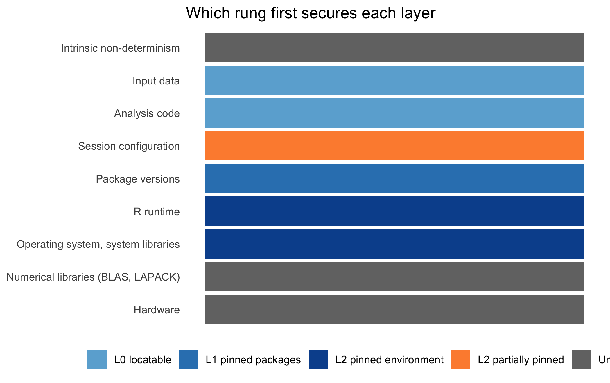
Now, which of these layers does common practice pin? The answer is sobering, and it motivates the entire book. A bare published script pins exactly one layer with any reliability, the analysis code, since the code is the file itself. If the reader is fortunate, it pins a second, the data, when it has been deposited alongside. Every other layer is left to whatever the next machine happens to provide. Figure 3.1 maps the stack against the rung of the ladder that first secures each layer. The reader will note that three layers, the hardware, the numerical libraries, and intrinsic non-determinism, are secured by no rung of the capture ladder at all.
library(ggplot2)library(tibble)stack <- tibble::tibble(layer =c('Hardware','Numerical libraries (BLAS, LAPACK)','Operating system, system libraries','R runtime','Package versions','Session configuration','Analysis code','Input data','Intrinsic non-determinism'),height =1:9,secured =c('Unpinned by any rung','Unpinned by any rung','L2 pinned environment','L2 pinned environment','L1 pinned packages','L2 partially pinned','L0 locatable','L0 locatable','Unpinned by any rung'))stack$secured <-factor( stack$secured,levels =c('L0 locatable', 'L1 pinned packages','L2 pinned environment', 'L2 partially pinned','Unpinned by any rung'))ggplot(stack, aes(x =reorder(layer, height),y =1, fill = secured)) +geom_col(width =0.9) +coord_flip() +scale_fill_manual(values =c('L0 locatable'='#6baed6','L1 pinned packages'='#3182bd','L2 pinned environment'='#08519c','L2 partially pinned'='#fd8d3c','Unpinned by any rung'='#737373'),name =NULL) +labs(x =NULL, y =NULL,title ='Which rung first secures each layer') +theme_minimal(base_size =11) +theme(axis.text.x =element_blank(),panel.grid =element_blank(),legend.position ='bottom')
Figure 3.1: The determinant stack, from the hardware at the base to the data at the top, colored by the rung of the ladder that first secures each layer. Package versions are secured at L1, the operating system and R runtime at L2, and the analysis code and data are merely locatable at L0. The session-configuration layer is only partially pinned at L2: the locale and the time zone are fixed, but the RNG kind, the contrasts, and the number of printed digits are not. Three further layers, the hardware, the numerical libraries, and intrinsic non-determinism, are pinned by no rung of the capture ladder.
Two features of the session-configuration layer deserve a word, because they are the layers most often forgotten by an analyst who has already adopted a lockfile and a container. The random-number kind is the more dangerous. An analysis that seeds its generator and draws a sample is reproducible only if the algorithm behind the seed is also fixed. The change of the default sample.kind in R 3.6.0 broke exactly this, silently, for every analysis that had set a seed under the old default. Given that simulation studies, multiple imputation, and bootstrap confidence intervals are staples of health research, the RNG kind is a first-order concern, not a footnote. The locale is the second. sort() and order() on a character vector depend on LC_COLLATE, and the parsing of a decimal mark depends on LC_NUMERIC. An analysis developed under one locale and re-run under another can therefore reorder a table or misread a number without any error.
NoteCheck your understanding: locating a failure on the stack
An epidemiologist reports that a colleague, re-running her cohort analysis, obtained an incidence rate identical to five decimal places but a different value in the sixth. The code, the data, the package versions, and the operating system were all identical. Which layer of the determinant stack is the most likely culprit, and is the discrepancy a bug?
NoteAnswer
Neither the code nor the data nor the pinned layers can be at fault, since all were identical. A discrepancy confined to the low-order digits is the signature of the numerical-library layer. The two machines used a different BLAS implementation, or the same one with a different thread count, and so the floating-point summations were reordered. It is not a bug in the analysis. It is the reason that byte-for-byte identity across different hardware is a stronger claim than number-for-number agreement on a fixed architecture. And it is a layer that no rung of the capture ladder pins.
3.5 The ladder: capture sets the level, validation confirms it
With the stack in view we can define the ladder. The central design idea, which we take from the framework this book uses and develop as a general principle, is that the features acting on reproducibility divide into two kinds that are constantly confused. Separating them is what makes an honest grade possible.
The capture axes fix inputs, and therefore set the level. There are two of them: the package backend, which pins the package layer, and the computational environment, which pins the operating system, the runtime, and the system libraries. Adding a capture feature raises the level; removing one lowers it. The validation layer confirms the captured level without capturing anything new. Its members are continuous integration, the dependency-consistency check, and the output-verification command. Removing a validation feature leaves a repository exactly as reconstructable as before; it only stops the automated checking. This is why continuous integration, which we develop in Chapter 12, is best understood as the harness that runs the verification rather than as a layer of reproducibility in its own right. Pinning is capture; re-running to confirm is validation.
The four rungs follow from this distinction. Levels L0 through L2 are reached by the capture axes, and L3 is reached by the validation layer. Table 3.1 states each rung, what it pins, the artifact that marks it, and what the rung means for a reader of health research.
library(tibble)library(knitr)ladder <- tibble::tibble(Level =c('L0 locatable','L1 pinned packages','L2 pinned environment','L3 verified'),`What is pinned`=c('Nothing computational; the source is under version control','The exact version of every R package','The operating system, the R runtime, and the system libraries as well','Nothing new; the recorded outputs have been regenerated and checked'),`Primary artifact`=c('A version-controlled repository','A lockfile such as renv.lock','A container image or a Nix environment','A passing verification run comparing regenerated outputs against a recorded baseline, re-run automatically by continuous integration'),`Health-research reading`=c('A reviewer can find the code but cannot yet rebuild it','A colleague installs the same packages the analysis used','The analysis yields the same numbers on a different machine','The reported table has been shown to regenerate, not merely asserted to'))knitr::kable(ladder)
Table 3.1: The reproducibility ladder used throughout this book. Each rung names what it pins, the primary artifact that marks it, and what reaching it means for a reader of health research.
Level
What is pinned
Primary artifact
Health-research reading
L0 locatable
Nothing computational; the source is under version control
A version-controlled repository
A reviewer can find the code but cannot yet rebuild it
L1 pinned packages
The exact version of every R package
A lockfile such as renv.lock
A colleague installs the same packages the analysis used
L2 pinned environment
The operating system, the R runtime, and the system libraries as well
A container image or a Nix environment
The analysis yields the same numbers on a different machine
L3 verified
Nothing new; the recorded outputs have been regenerated and checked
A passing verification run comparing regenerated outputs against a recorded baseline, re-run automatically by continuous integration
The reported table has been shown to regenerate, not merely asserted to
The rungs are cumulative. An L2 analysis is also locatable and package-pinned; the label names the highest rung reached. The transition that matters most for a first-year student to internalize is the one between L1 and L2. A lockfile alone, the L1 artifact, pins the packages but not the R version, the operating system, or the system libraries a package links against. A lockfile restored under a different R version may fail to install or, more insidiously, may install and behave differently. The container image, the L2 artifact, fixes what the lockfile cannot. The two are complements, not substitutes, and a genuinely pinned-environment analysis carries both.
Where does the ladder come from, and is it arbitrary? It is not. It consolidates several graded views of reproducibility that the literature has offered in different vocabularies. Peng (2011) arranged computational work along a spectrum, from the merely published, through code available, code and data available, and linked and executable, to full replication. Our L0, L1, and L2 track the lower and middle reaches of that spectrum. The artifact-review badges used by the ACM and several computing venues express a related ordering, from artifacts that are available, through artifacts evaluated as functional and then reusable, to results independently reproduced (Association for Computing Machinery, 2020). Our L3 is the analogue of the ‘Results Reproduced’ badge. The correspondence is close but not exact. The ‘functional’ and ‘reusable’ badges grade how well an artifact is documented and exercised rather than the package-versus-environment pinning depth that separates L1 from L2, so the middle rows are analogies rather than alignments. The contribution of the L-scheme is not a new definition of reproducibility but a mapping of these graded views onto artifacts a tool can detect. The point is that the level of a repository can then be determined mechanically and reported honestly, rather than asserted by its author.
NoteCheck your understanding: capture or validation?
A laboratory adds a continuous-integration workflow that rebuilds its compendium and runs the tests on every push. A colleague objects that this cannot improve reproducibility, because it pins no new layer of the determinant stack. Is the colleague correct, and has the laboratory wasted its effort?
NoteAnswer
The colleague is correct on the narrow point and wrong on the conclusion. Continuous integration is a validation feature, not a capture feature: it pins no new layer, and removing it would leave the compendium exactly as reconstructable as before. What it adds is confirmation. It re-runs the captured analysis in a clean environment that carries none of the author’s undeclared state. It therefore catches the silent decay that a captured-but-never-retested analysis suffers, and the ‘works on my machine’ failure at its source. The laboratory has moved from L2, a pinned environment asserted to reproduce, toward L3, a pinned environment shown to reproduce. That is the whole purpose of the capture-versus-validation distinction.
3.6 Reproduced, replicated, and a warning about the words
The ladder grades re-execution, and re-execution is only one of the things the word ‘reproducibility’ is made to carry. A first-year student must fix the terms before reading the literature, because the same two words are attached to opposite meanings across the sources a reader will meet.
The National Academies, in their 2019 consensus report, adopt the distinction this book follows (National Academies of Sciences, Engineering, and Medicine, 2019). Reproducibility is obtaining consistent computational results using the same input data, the same code, and the same conditions of analysis: it is a statement about re-execution, and it is what the ladder grades. Replicability is obtaining consistent results across studies aimed at the same question, each with its own data: it is a statement about the robustness of a scientific finding. The two are independent. A result can be perfectly reproducible and entirely wrong, if the code faithfully regenerates a mistaken number every time. And a finding can replicate across laboratories while no single analysis in the set is computationally reproducible. Leek and Peng press exactly this point, that a reproducible analysis can still be wrong, and that reproducibility is therefore a floor and not a ceiling (Leek & Peng, 2015). Patil, Peng, and Leek go further and offer a statistical framing of the distinction, casting replication as a question about the agreement of estimates across studies rather than about the re-running of code (Patil et al., 2016).
Here is the warning. The current ACM artifact-badge vocabulary, in its 2020 revision, agrees with the National Academies usage rather than inverting it (Association for Computing Machinery, 2020). Under both conventions, ‘Reproduced’ denotes obtaining a prior result using the author’s own artifacts and the same setup, and ‘Replicated’ denotes obtaining it independently, with a different team and a new setup. The genuine word-swap that trips students belongs to two other places. One is the pre-2020 ACM badging, which attached the two words in the opposite direction along the re-execution axis. The other is some biomedical and field usages, which a reader may still encounter, where ‘reproduce’ names an independent study rather than a re-run. A reader who carries the sense of the words from one of those older documents into a current one will be misled, silently and without any error to warn them, in exactly the manner of a shifted package default. This book fixes the meaning and states it once: throughout, L3 denotes the ACM ‘Results Reproduced’ sense, which now coincides with the National Academies reproducibility sense. That sense is that the captured analysis, rebuilt from its pinned definition and re-run, regenerates its own recorded outputs. It is deliberately not replication in the sense of an independent study on new data, which no software framework can supply. When the reader meets ‘reproduced’ or ‘replicated’ in a journal’s author instructions or a venue’s badging policy, the first task is to determine which convention that document uses. The word alone does not tell them.
ImportantThe honest level
A reproducibility claim must be matched to the level actually reached, and never asserted above it. An analysis that carries a lockfile but no container is at L1, and a manuscript that describes it as ‘fully reproducible’ overstates by two rungs. The remedy is not modesty for its own sake but accuracy: state the rung, name the artifact that marks it, and name the layers left exposed. ‘This analysis is pinned at L2, with the RNG kind fixed and the input data checksummed; it has not been verified under zzc verify and so is not claimed at L3’ is a sentence that a reviewer can act upon. ‘Fully reproducible’ is not.
3.7 Two numbering schemes, and which this book uses
A reader who consults the documentation of the framework this book uses will encounter a second numbering scheme, and the collision is a genuine source of confusion that we disarm here rather than leave to chance.
The framework’s teaching materials include a vignette that presents a five-level ramp: Level 1, a basic R project with manual package management; Level 2, the addition of renv; Level 3, the addition of Docker; Level 4, the addition of unit testing; and Level 5, the addition of continuous integration. That scale counts which tools a project has adopted, and it is a pedagogical on-ramp, meant to be walked from the bottom as a project matures. It is a useful thing, but it is not the scale of this book.
The scale of this book is the architectural ladder of the preceding sections, L0 through L3, and it grades something different: how far down the determinant stack a result has been locked, and whether the lock has been verified. The two axes are related but not identical. Adopting renv (the tool scheme’s Level 2) is what lifts a project to L1. Adopting a container (the tool scheme’s Level 3) is what lifts it to L2. The tool scheme’s testing and continuous-integration levels belong to the validation layer that reaches L3. But one can imagine a project that has adopted every tool and still verified nothing, and the architectural ladder, not the tool count, is what tells the reader whether the result has been shown to reproduce.
To avoid ambiguity we adopt a single convention. This book uses the L0 to L3 architectural ladder throughout, in every chapter and every worked example. Where the framework’s own documentation speaks of ‘Level 1’ through ‘Level 5’, it is using the tool-adoption ramp, and the reader should read it as such and not conflate it with our L0 to L3. When we write a bare ‘L2’, we always mean the architectural rung.
3.8 The ladder grades every archetype
It would be a mistake to read the ladder as a scale for manuscripts alone. A research compendium, as Chapter 5 develops in full, comes in several archetypes, and the ladder grades each of them by the same means and to the same rungs.
A data-analysis project and a scholarly manuscript are the familiar cases, and for them the reading is the one given above: the lockfile lifts to L1, and the container lifts to L2. The verification run, for a manuscript, re-renders the report and compares its figures and tables against a recorded baseline, and this is what lifts it to L3. An R package, by contrast, has no report to render. Its L3 verification is instead the passing of R CMD check and its test suite in a clean environment, rather than the regeneration of a manuscript, though the pinning of its packages and its environment is otherwise identical. A simulation study reaches the same rungs by the same artifacts, but its exposure on the session-configuration layer is acute, because its outputs are functions of the random-number stream. An unseeded or wrongly seeded simulation can sit at L2, with a perfectly pinned environment, and still fail to reproduce. For this archetype, the discipline of fixing the RNG kind and the seed is the difference between a nominal L2 and a real one. A blog renders many posts rather than one report. Its L3 verification is the successful rebuild of the whole site from its pinned environment, and the ladder applies post by post exactly as it applies to a single manuscript.
The lesson is that the ladder is a property of the determinant stack, which every archetype shares, and not of any particular directory layout. A package or a blog reaches L2 by the same container that an analysis project does, and reaches L3 by a verification appropriate to what it produces.
3.9 No framework pins the whole stack
We end the exposition where honesty requires, with the boundary of the guarantee. It would be incoherent to spend a chapter teaching that a reproducibility claim must be matched to the level actually reached, and then to imply that reaching L2 or L3 pins the entire determinant stack. It does not, and no present framework does.
By its own published accounting, the framework this book uses robustly pins something like four of the ten determinants: the operating system and system libraries (as strongly as its base image is pinned), the R package versions (nominally, through the lockfile), the locale and time zone, and the source code. It leaves others to convention or to the base image: the random-number kind is not pinned by default, the BLAS and LAPACK threading regime is inherited from the base image and neither pinned nor documented, the integrity of external data is recorded by provenance but not by checksum, and the fonts and the graphics device are pinned only for some profiles. These are not defects peculiar to one tool. They are the layers that the whole class of integrative frameworks currently leaves exposed, and an honest L2 or L3 claim names them rather than papering over them. The reader will therefore find, at each rung of the ladder in the chapters ahead, an explicit account of what is secured and what remains exposed. Reach plus honesty about the boundary of that reach is the standard this book holds every effort to, including the framework it teaches.
3.10 Worked example
To make the ladder concrete, consider a single analysis walked up all four rungs. A biostatistician has a folder containing analysis.R, which reads cohort.csv, fits a Cox model with the survival package, and writes a hazard ratio to results.csv. We shall place it on the ladder and name each transition.
At the start the folder is on the analyst’s laptop and nowhere else. It is at no rung of the ladder at all, because it cannot even be found by a second person. The first act, placing the folder under version control and pushing it to a repository, lifts it to L0, locatable. A reviewer can now find analysis.R and read it. Nothing computational is pinned; a reviewer who runs it will install whatever version of survival happens to be current, which may not be the version the analyst used.
The analyst now runs renv::init() and renv::snapshot(), which we develop in Chapter 6. This writes a renv.lock recording that the analysis used survival version 3.5-7, together with the exact version of every other package in the closure. The folder is now at L1, pinned packages. A colleague who restores from the lockfile obtains the same survival the analyst used. But the colleague’s laptop runs a newer R and a different operating system, and one of the packages links against a system library that is absent, so the restore fails to build.
To close that gap the analyst adds a container, developed in Chapter 7, built from a dated rocker base image pinned by its content digest. The image carries a fixed operating system, a fixed R, and the system libraries the packages need, and the lockfile restores inside it. The folder is now at L2, pinned environment. It will build and run identically on the colleague’s laptop, on a reviewer’s, and on a server. The analyst also sets the RNG kind and a seed in the project .Rprofile, because the analyst computes bootstrap confidence intervals for the hazard ratio, closing a session-configuration exposure that L2 does not close by default.
Finally the analyst adds a verification step, developed in Chapter 12, that rebuilds the image, re-runs analysis.R, and compares the regenerated results.csv against a recorded baseline. The first time it runs it passes, and a continuous-integration service re-runs it on every change. The folder is now at L3, verified: the reported hazard ratio has been shown to regenerate, not merely asserted to. The honest reproducibility statement for the paper now writes itself, naming the rung, the artifacts, and the one layer, the cross-architecture numerical determinism of the bootstrap, that remains outside the guarantee.
3.11 Collaborating with an LLM
A large language model is a capable assistant for reasoning about levels. But it is confident in a register that this chapter has just taught the reader to distrust, and its confidence is not calibrated to the honest level. The following triples illustrate productive prompts and the verification each demands.
Prompt. ‘Here is my project directory listing. What reproducibility level has it reached on the L0 to L3 ladder, and what would it take to reach the next rung?’
Watch for. The model will read the presence of a renv.lock as L1 and a Dockerfile as L2, which is the right heuristic. But it cannot tell from a listing whether the lockfile is current, whether the image is pinned by a mutable tag or an immutable digest, or whether a verification run has ever passed. It may report L3 on the strength of a continuous-integration file that has never been run green.
Verification. Confirm each rung against the artifact itself, not its filename. For L1, check that the lockfile is in step with the code. For L2, check that the base image carries a digest and that the library is not shadowed by a bind mount. For L3, find an actual passing verification run. The presence of a file is capture asserted; a green run is validation observed.
Prompt. ‘Draft the reproducibility statement for my methods section.’
Watch for. The model gravitates to the phrase ‘fully reproducible’, which this chapter has argued is almost never an honest claim. It will also tend to conflate ‘reproducible’ and ‘replicable’ in the National Academies sense, or to use the ACM sense without saying so.
Verification. Rewrite the draft to name the specific rung, the artifacts that mark it, and the layers left exposed, and to state which convention of ‘reproduced’ is meant. Reject any sentence you could not defend to a reviewer who ran the code.
Prompt. ‘My simulation gives slightly different numbers each time even inside the container. Why, and is it a bug?’
Watch for. The model may propose plausible but wrong culprits, a package version or an operating-system difference, that the container has already pinned. It may also not distinguish an unseeded RNG (a real defect) from low-order-digit variation due to BLAS threading (an inherent limit at L2).
Verification. Trace the discrepancy to a layer of the determinant stack. If the numbers differ in all digits, look to the RNG kind and the seed, which the analyst controls. If they differ only in the low-order digits, suspect the numerical-library layer, which no rung of the capture ladder pins, and decide whether that residual matters for the inference at hand.
3.12 Exercises
For an analysis of your own, list the nine or ten layers of the determinant stack and, for each, state whether your current setup pins it, and by what artifact. Identify the lowest layer you have left unpinned.
Take a published paper in your field that provides code. Without running it, place it on the L0 to L3 ladder from the materials the authors supply, and write the one-sentence reproducibility statement the paper should have carried.
Explain, to a colleague who believes that a Docker image makes an analysis ‘fully reproducible’, two determinants that the image does not pin and one circumstance in which each would cause two runs to disagree.
The framework’s documentation grades a project ‘Level 4’ on its five-level tool-adoption scale. State what this does and does not tell you about the project’s rung on the L0 to L3 architectural ladder, and name one artifact you would inspect to settle the question.
A colleague reports that a finding ‘replicated’ in a second cohort. A reviewer reads this as an ACM artifact badge and asks for the container. Explain the miscommunication in terms of the two conventions for the word, and state which sense the colleague almost certainly intended.
Construct a small simulation in R that draws a sample under a fixed seed, and show that changing the RNG kind with RNGkind() changes the draw while leaving the seed unchanged. Explain which layer of the determinant stack this demonstrates and why a container alone would not protect against it.
3.13 Solutions
Attempt an exercise before expanding its solution. Two of these ask the reader to work with an analysis or a paper of their own, so they have no single correct answer; for those the box says what a good answer establishes.
NoteExercise 1
No single correct answer. What a good answer establishes is that the reader can name the layers in order and attach an artifact, or an admission, to each.
Working up from the base: hardware, pinned by nothing short of running on the same machine; numerical libraries, pinned by the container image if it fixes the BLAS, and otherwise not at all; operating system and system libraries, pinned by the container image; R runtime, pinned by the container image, and merely recorded by the lockfile’s R block; package versions, pinned by renv.lock; session configuration, partly pinned by the image through the locale and the time zone, and not pinned at all for the RNG kind, the contrasts, and the printed digits; analysis code, pinned by version control; input data, pinned by a checksum or an archived deposit, and often only locatable; and intrinsic non-determinism, such as parallel reduction order, pinned by nothing.
Most readers find their lowest unpinned layer is either the numerical libraries or the session configuration, and both answers are common and honest. A reader who finds their lowest unpinned layer is the input data has discovered something more urgent than anything this chapter teaches, because the analysis is not reconstructable at all.
NoteExercise 2
No single correct answer. What a good answer establishes is that the rung is read off the deposited artifacts, not off the quality of the paper or the reputation of the authors.
The procedure is mechanical. Is there code and data that can be located? That is L0. Is there a lockfile, or an equivalent exact version record? That is L1. Is there a container recipe, or another artifact pinning the runtime and the system libraries? That is L2. Is there evidence that the outputs were regenerated from the pinned definition, a CI log, a verification report, recorded output hashes? That is L3. Stop at the highest rung for which an artifact is actually present.
The reproducibility statement should then claim that rung and no more. For the common L0 case: ‘The analysis code and the derived dataset are deposited at [location]. The software environment was not recorded, so re-execution may require package versions that differ from those used here.’ The second clause is the part most papers omit, and it is the part that makes the statement honest rather than merely modest.
NoteExercise 3
Two determinants an image does not pin, with a circumstance for each.
The numerical libraries, when the image does not fix them. An image built on a base that links against a BLAS chosen at run time, or one run on hosts that expose different thread counts, will reorder floating-point summations. Two runs of the same image on two machines can then return an incidence rate agreeing to five decimal places and differing in the sixth. The image pinned the software and not the arithmetic beneath it.
The session configuration, specifically the RNG kind. An image fixes the R version, and the R version determines the default sampler, so this exposure is narrower than it first appears. It bites when the analysis sets RNGkind() itself, or inherits it from a project .Rprofile that is mounted rather than baked in, or when a package changes the generator as a side effect. Two runs then draw different samples from the same seed, and a bootstrap interval moves.
A third acceptable answer is the input data: an image mounting a host directory reproduces the environment and not the extract, so a changed file underneath produces a different result with the image unchanged. A fourth is intrinsic non-determinism from parallelism, where the reduction order of a parallel sum varies run to run on the same machine.
The general form of the answer is that a container pins the environment and the environment is not the whole stack. It is the L1-to-L2 step, not the whole ladder.
NoteExercise 4
‘Level 4’ on the framework’s scale means the project has adopted a particular set of tools: an R project, renv, Docker, and unit testing. It is a statement about tool adoption, and it is read from the bottom up, so Level 4 implies the first three as well.
What it tells you about the architectural ladder is therefore quite a lot, but indirectly and with one gap. The presence of renv implies the machinery for L1; the presence of Docker implies the machinery for L2. What it does not tell you is whether any of it has been verified, because the tool scale counts adoption and the architectural ladder grades locking and verification. A project can hold every tool in the list and have never rebuilt from its pinned definition, in which case it sits at L2 and is asserted rather than shown to reproduce. L3 is the tool scale’s Level 5 territory, and Level 4 is below it.
The artifact to inspect is the continuous-integration record: a log showing that the container was rebuilt from the recipe and the analysis re-run, and its outputs checked against recorded values. Absent that, the honest reading of ‘Level 4’ is L2. Inspecting renv.lock and the Dockerfile tells you the capture artifacts exist; only the CI record tells you the capture works.
NoteExercise 5
The colleague almost certainly meant the National Academies sense: a second cohort, collecting its own data, found a consistent result. That is replication, a statement about the durability of the finding, and it is the sense in which the word is ordinarily used in health research.
The reviewer read it in an artifact-badging frame, where the pair of words attaches to re-execution rather than to new data. Under the current 2020 ACM vocabulary the two conventions actually agree, so the reviewer’s request is not simply a misreading of the current standard. The miscommunication traces to one of two places: the pre-2020 ACM badging, which attached the two words in the opposite direction, or a field usage in which ‘reproduce’ names an independent study rather than a re-run. A reviewer carrying the sense of the words from an older document into a current one is misled silently, with no error to warn them.
The practical resolution is that the container request is a category error given what the colleague did. A container would let the reviewer re-execute the original analysis, which is not what the colleague claimed and not what a second cohort demonstrates. The colleague should answer by naming the convention, stating that the second cohort collected its own data, and offering the artifact that actually matches the claim, which is the second cohort’s own analysis code.
NoteExercise 6
The demonstration is the worked example of Chapter 2 in miniature.
The two calls share a seed and return different draws. Restoring the original generator afterward matters, since RNGkind() sets session state that would otherwise persist and quietly affect everything downstream.
The layer demonstrated is the session configuration layer, which sits above the package versions and below the analysis code. It is the layer this chapter singles out as only partially pinned at L2: an image fixes the locale and the time zone, and the R version it carries fixes the default sampler, but the RNG kind, the contrasts, and the number of printed digits are all settable from inside the session and are not properties of the image.
A container alone would not protect against this because the change is made by the analysis, inside the container, after the environment is fixed. Two runs of the identical image produce different draws if the code sets the sampler differently, or if a mounted .Rprofile does. The protection is not a heavier container but an explicit declaration: set RNGkind() in the analysis, record it alongside the seed, and treat it as part of the analysis code rather than part of the environment.
3.14 Further reading
National Academies of Sciences, Engineering, and Medicine (2019) is the National Academies consensus report that fixes the reproducible-versus-replicable terminology this book follows; read its opening chapter for the definitions and the reasoning behind them.
Peng (2011) introduces the reproducibility spectrum that our ladder consolidates, and argues for reproducibility as a minimum standard when full replication is impractical; the earlier Peng (2009) applies the idea to epidemiology directly.
Leek & Peng (2015) makes the case that reproducibility is a floor and not a ceiling, and Patil et al. (2016) offers a statistical framing of the distinction between reproducing a computation and replicating a finding.
Association for Computing Machinery (2020) documents the artifact-review badges whose ‘available’, ‘functional’, ‘reusable’, and ‘reproduced’ ordering our ladder maps onto; read it alongside National Academies of Sciences, Engineering, and Medicine (2019) to see how the 2020 revision aligns the two vocabularies.
The Turing Way Community (2022) crosses the reproducibility axis with a what-varies axis, same or different data against same or different analysis, and is the most accessible community handbook for a first-year student.
For the determinant stack and the capture-versus-validation distinction as a framework applies them, Sandve et al. (2013) and Wilson et al. (2017) give the practices, the former stressing the recording of random-number seeds and exact versions that the ladder’s session-configuration layer names.
Leek, J. T., & Peng, R. D. (2015). Reproducible research can still be wrong: Adopting a prevention approach. Proceedings of the National Academy of Sciences, 112(6), 1645–1646. https://doi.org/10.1073/pnas.1421412111
National Academies of Sciences, Engineering, and Medicine. (2019). Reproducibility and replicability in science. The National Academies Press. https://doi.org/10.17226/25303
Patil, P., Peng, R. D., & Leek, J. T. (2016). A statistical definition for reproducibility and replicability. bioRxiv, 066803. https://doi.org/10.1101/066803
Sandve, G. K., Nekrutenko, A., Taylor, J., & Hovig, E. (2013). Ten simple rules for reproducible computational research. PLOS Computational Biology, 9(10), e1003285. https://doi.org/10.1371/journal.pcbi.1003285
The Turing Way Community. (2022). The TuringWay: A handbook for reproducible, ethical and collaborative research. Zenodo. https://doi.org/10.5281/zenodo.3233853
Wilson, G., Bryan, J., Cranston, K., Kitzes, J., Nederbragt, L., & Teal, T. K. (2017). Good enough practices in scientific computing. PLOS Computational Biology, 13(6), e1005510. https://doi.org/10.1371/journal.pcbi.1005510