plot_determinant_stack(
  title = 'A diagnosis, not yet a capture or a validation')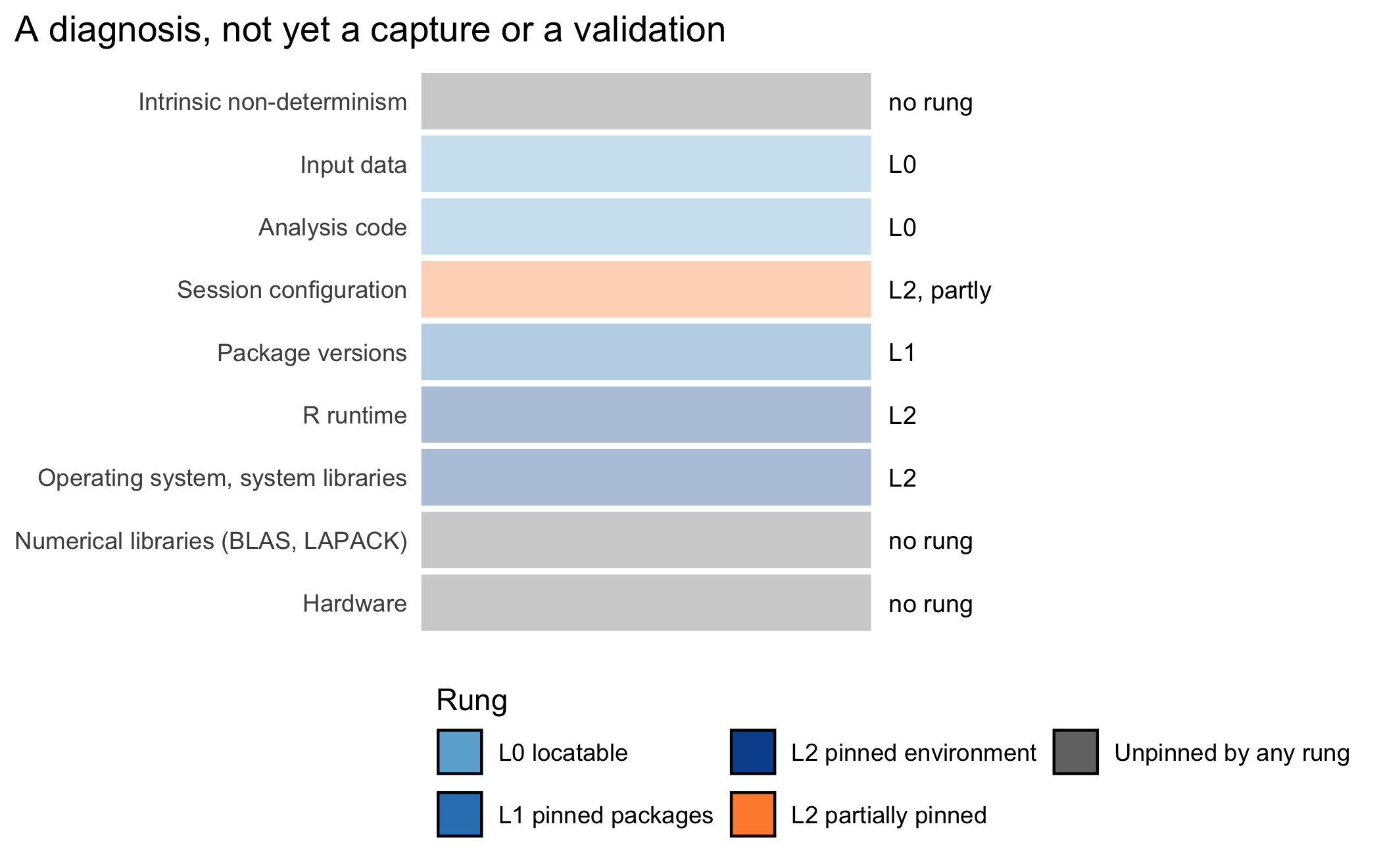
More than 70% of researchers have tried and failed to reproduce another scientist’s experiments, and more than half have failed to reproduce their own experiments.
Monya Baker, 1,500 Scientists Lift the Lid on Reproducibility (2016)
By the end of this chapter you will be able to look at a re-execution failure like the auditor’s below and say, concretely, whether the fault is statistical or computational. You will also be able to name the specific silent default most likely responsible, and to place the original analysis on the ladder this book develops in full in Chapter 3.
Consider a situation that every quantitative health scientist eventually meets. A biostatistician on a clinical-trial team runs the primary analysis and obtains the treatment effect and its confidence interval. The biostatistician exports the table that will anchor the regulatory submission and files the script. Two years later, during an audit, an inspector asks that the analysis be regenerated from the archived code and data. On a fresh machine the script errors on the first library() call. Once the missing package is located and installed, the analysis runs. The point estimate has moved in the third decimal place, however, and one confidence interval no longer excludes the null. Nothing in the statistical reasoning was wrong. What failed was everything around the statistics: a package that changed beneath the code, a default that shifted between releases of R, a system library present on the first machine and absent on the second.
This book exists to prevent that failure, and in this chapter we shall establish that the failure is real, common, and specifically computational. In a health science, a result that cannot be regenerated cannot be audited. An analysis that a regulator cannot reproduce is one a regulator may decline to trust. A clinical recommendation built on a number that no one can recompute rests on faith rather than evidence.
Throughout the book we place an analysis on a four-rung ladder, and we shall begin to use its vocabulary at once. An analysis is L0, locatable, when it is under version control and its source can be found, but nothing computational is pinned. It is L1, pinned packages, when the exact version of every package is fixed by a lockfile. It is L2, pinned environment, when the operating system, the language runtime, and the system libraries are fixed as well, usually inside a container. It is L3, verified, when the recorded computational outputs have been shown to regenerate within a stated tolerance from a clean rebuild, checked by a baseline test. The auditor’s failure above is the failure of an analysis that reached, at best, L0: the code could be found, and nothing else about the computation had been fixed. The ladder is developed in full in Chapter 3; here we use it only to name what was missing.
The chapter proceeds as follows. After locating the chapter on the determinant stack and setting out the judgments that belong to the analyst, we review the evidence that re-execution fails, separating replication studies from re-execution studies. We then fix three terms that are often confused: reproducibility, replicability, and robustness. Next we show, using two silent defaults in R itself, why the failures are computational and not statistical. We also argue that a reproducible analysis can still be wrong. Lastly, a worked example compares the same seed under two samplers, and the running cohort makes one silent default explicit in its loading function.
This chapter diagnoses rather than pins, and since Chapter 3 has not yet drawn the distinction between capturing a layer and validating one, the figure below claims neither. The prose names the layers of the determinant stack most responsible for the re-execution failures the evidence below documents. These are the R runtime itself and the session configuration riding on top of it. The RNG-kind comparison below and the stringsAsFactors comparison in ‘The cohort, continued’ each show an unpinned layer behaving exactly as badly as the chapter claims. No lockfile, no container, and no baseline test appears until later chapters, so Figure 2.1 highlights nothing. Its point is the blank stack itself, which Chapter 3 gives a name to and every later chapter’s figure will mark.
plot_determinant_stack(
title = 'A diagnosis, not yet a capture or a validation')Before turning to the evidence, we note three judgments at the center of this chapter that belong to the analyst and are automated by no tool.
Naming the failure mode. When a result will not regenerate, or regenerates differently, the analyst must decide what kind of discrepancy it is. It may be statistical (the method was inappropriate, the inference was misdrawn) or computational (the code is sound but its environment has shifted). The remedy differs entirely by case.
Matching the claim to the level reached. A reproducibility claim is a scientific claim and must be calibrated to evidence. The analyst decides, and states honestly, which rung of the ladder an analysis has actually reached, and resists the temptation to assert a level higher than the one secured.
Deciding what must be pinned. Not every determinant matters equally for every analysis. A simulation study lives or dies by its random-number configuration; a geospatial pipeline depends on system libraries that a survey analysis never touches. Judging which layers of the stack are load-bearing for the analysis at hand is a decision the analyst makes before any tool is invoked.
New to these terms? Each is defined again on first use.
set.seed) is the fixed starting point that makes a random draw repeatable; the RNG kind is the generator algorithm that turns that seed into numbers, and its default has changed across R versions.We begin with the large replication studies, because they set the scale of the problem. We then turn to the narrower and, for our purposes, more damning studies that isolate the computational failures.
In psychology, the Open Science Collaboration re-ran one hundred published studies. Its teams judged the original finding replicated in only thirty-nine of them, and only thirty-six percent of the replications reached statistical significance (Open Science Collaboration, 2015). In preclinical oncology, Begley and Ellis, working from within industry, reported that only six of fifty-three landmark findings could be reproduced, a success rate close to one in ten (Begley & Ellis, 2012). These figures were not, at first, universally believed. But the suspicion that the published literature was less solid than it appeared already had a theoretical footing. Ioannidis had argued, given the prevailing rates of low statistical power, analytical flexibility, and publication bias, that most published research findings are false (Ioannidis, 2005). When Baker later surveyed more than fifteen hundred researchers for Nature, a majority agreed that science was facing a reproducibility crisis. More than seventy percent reported that they had tried and failed to reproduce another scientist’s experiments (Baker, 2016).
These are, for the most part, failures of replication, at the scientific end of a spectrum we shall shortly define, and their causes are many. But a growing body of work isolates the specifically computational failures. Here the question is not whether a finding holds up in a new sample, but merely whether the original analysis can be made to run a second time. The evidence there is starker, because the failures are more avoidable. Trisovic and colleagues re-ran more than nine thousand R files deposited alongside published articles in the Harvard Dataverse. Roughly one in four executed without error, before any question of whether the output matched the published result (Trisovic et al., 2022). Saju and colleagues examined R code supplements archived on the Open Science Framework. Only about a quarter of the R scripts ran without error, even in environments the authors rebuilt, and only one project in six ran in full. Close to ninety-nine percent of the projects carried no formal description of their dependencies at all (Saju et al., 2025).
We see, then, that the replication studies tell us that scientific findings are fragile. The re-execution studies tell us something more specific and more remediable, namely that a large fraction of published analyses cannot be regenerated even in principle. The reason is that the computational scaffolding needed to run them was never captured. The tooling in this book addresses the second failure.
Before proceeding we need to fix our terms. The vocabulary of this field is genuinely contested, and a reader who does not fix it will be confused by the literature. Goodman and colleagues surveyed the usage and found that the same words carry opposite meanings in different research communities: one field’s ‘reproducibility’ is another field’s ‘replication’ (Goodman et al., 2016). We adopt the distinctions of the National Academies, whose 2019 consensus report offers the settlement most widely followed in the health sciences (National Academies of Sciences, Engineering, and Medicine, 2019).
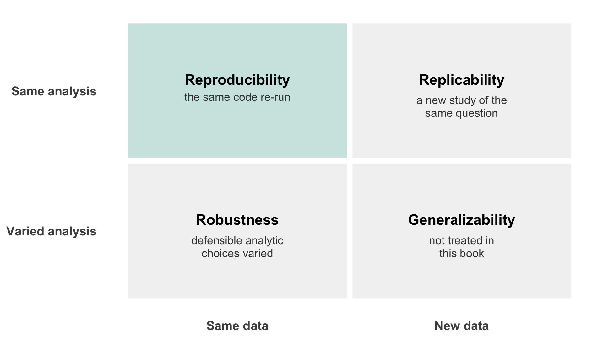
Reproducibility is obtaining consistent computational results using the same input data, the same computational steps, methods, and code, and the same conditions of analysis. It is a statement about re-execution, and it is the subject of this book. Replicability is obtaining consistent results across studies aimed at the same question, each collecting its own data. It is a statement about the durability of a scientific finding. To these two the wider literature, notably the Turing Way (The Turing Way Community, 2022), adds a third, robustness, obtaining consistent conclusions from the same data when the analytical choices are varied within the range a competent analyst would defend. The three are independent. An analysis can be perfectly reproducible and entirely wrong, faithfully regenerating the same mistaken number on every machine. A finding can replicate across laboratories while no single analysis in the set is computationally reproducible. And a result can be reproducible yet fragile to a defensible change in model specification.
How, then, are the three terms to be kept apart? They sort cleanly once we notice that each answers the same question: what was held fixed, the data or the analysis. Figure 2.2 lays the possibilities out as a grid, a presentation the Turing Way has made the common one (The Turing Way Community, 2022). The fourth cell, in which both the data and the analysis change, is generalizability. We name it here for completeness and do not treat it.
library(ggplot2)
library(tibble)

grid <- tibble(
  data     = rep(c('Same data', 'New data'), each = 2),
  analysis = rep(c('Same analysis', 'Varied analysis'), 2),
  term = c('Reproducibility',
           'Robustness',
           'Replicability',
           'Generalizability'),
  gloss = c('the same code re-run',
            'defensible analytic\nchoices varied',
            'a new study of the\nsame question',
            'not treated in\nthis book'),
  focus = c(TRUE, FALSE, FALSE, FALSE)
)

grid$data <- factor(grid$data, levels = c('Same data', 'New data'))
grid$analysis <- factor(grid$analysis,
                        levels = c('Varied analysis', 'Same analysis'))

ggplot(grid, aes(x = data, y = analysis)) +
  geom_tile(aes(fill = focus), color = 'white', linewidth = 2) +
  geom_text(aes(label = term), vjust = -0.6,
            fontface = 'bold', size = 3.9) +
  geom_text(aes(label = gloss), vjust = 1.25, size = 3,
            lineheight = 0.95, color = 'grey25') +
  scale_fill_manual(values = c('TRUE' = '#cfe6e3',
                               'FALSE' = '#f2f2f2'),
                    guide = 'none') +
  labs(x = NULL, y = NULL) +
  theme_minimal(base_size = 10) +
  theme(
    panel.grid = element_blank(),
    axis.text = element_text(face = 'bold', size = 9.5)
  )
The idea that computational work should be reproducible in the narrow, re-execution sense is older than the current crisis. It is usually traced to Claerbout and his colleagues in geophysics. In the early 1990s they built their books and reports so that every figure could be rebuilt from the archived code and data (Buckheit & Donoho, 1995; Claerbout & Karrenbach, 1992). Their standard was demanding. The phrasing that has become the field’s motto is Buckheit and Donoho’s paraphrase of it (Buckheit & Donoho, 1995; Claerbout & Karrenbach, 1992): the published article is merely the advertisement of the scholarship, and the scholarship itself is the full computational apparatus that produced the figures.
Reproducibility so understood is a spectrum. Peng arranged computational work along a scale, from the merely published, through code available, code and data available, and linked and executable, to fully replicable. He argued that reproducibility can serve as a minimum standard for judging a scientific claim when full independent replication is not possible (Peng, 2011; Peng et al., 2006). We take from Peng the idea that reproducibility comes in degrees, and that honesty about which degree one has reached is itself a scientific virtue. We shall develop that idea into the levels ladder of Chapter 3.
We now ask why re-execution fails, and the reasons point directly at the remedy. Consider two changes to R itself, each silent, each an improvement, and each capable of altering a published result without any error or warning to announce it.
In R 3.6.0, released in 2019, the default algorithm that turns a seed into a random sample was corrected. The old sampler introduced a slight bias in sample(); the new one removed it. The consequence for reproducibility is direct. Code that set a seed and drew a sample obtained one sequence of draws before the release and a different sequence after it, with identical code and an identical seed (R Core Team, 2019). Every bootstrap resample, every cross-validation fold assignment, and every permutation test built on sample(), directly or through a function that calls it, draws differently under the new default than under the old one. A simulation that draws from rnorm(), rpois(), or another generator that does not route through sample() is unaffected; the 2019 correction touched one generator, not every source of randomness in R.
Then, in R 4.0.0, released in 2020, the stringsAsFactors default flipped from TRUE to FALSE. Reading a data frame now silently produced character columns where it once produced factors. This affected any code that depended on factor-specific behavior, such as the ordering of levels or a function that requires a factor (R Core Team, 2020). Neither change was a bug; both were deliberate improvements. Both would nonetheless break the exact reproduction of an analysis written under the old default, and neither would say a word.
To these language-level shifts we must add the steadier erosion of package churn, the phenomenon by which working code rots as the packages beneath it are updated. A modern analysis may depend on dozens or hundreds of packages, each with its own release history and its own breaking changes. Much of this churn, along with missing files and hard-coded paths, is what Trisovic and colleagues measured when they found that most deposited R scripts did not run when re-executed, often years after the original deposit (Trisovic et al., 2022).
These are instances of a general phenomenon that we shall develop fully in Chapter 3. A computational result depends not only on the code and the data but on a stack of determinants beneath them. The stack includes the operating system and its system libraries, the numerical libraries that implement linear algebra, the language runtime, and the exact versions of every package. It also includes the session configuration (the random-number kind, the contrasts, the number of printed digits, the locale and time zone) and, underneath all of it, the hardware. A published script pins almost none of these. It records the analysis logic and, if the reader is fortunate, the data. The remaining layers are left to whatever the next machine happens to provide. Reproducibility fails in the gap between what the script fixes and what the result depends on. The organizing question of this book is how far down that stack a given effort has actually reached.
This diagnosis, that the failures are computational rather than statistical, is what makes the problem tractable. A statistical error requires a scientific judgment to correct; a computational failure requires only that the determinant stack be captured, layer by layer, so that the same computation can be run again. Computational hygiene of that kind can be taught, tooled, and enforced.
The same exposure applies to every kind of computational output, including outputs with no polished manuscript. A research compendium comes in several archetypes, developed in full in Chapter 5: a data-analysis project, a scholarly manuscript, an R package, a simulation study, and a blog of many rendered posts. Each varies the directory layout, whether a rendered report exists at all, and which validation gates apply. However, all share the same determinant stack, and so all are exposed to the same silent shifts. An R package with no report to render can still be broken by a changed sample.kind. A simulation study that resamples, permutes, or randomizes through sample() is more exposed to the RNG change than any manuscript, since its whole output is a function of those draws. And a teaching blog that renders forty posts inherits the churn of every package any post loads.
Nothing in this book claims that a reproducible analysis is a correct one. The point is pressed by Leek and Peng, who observe that reproducibility guarantees only that a computation can be regenerated, not that the computation was the right one to perform (Leek & Peng, 2015). A script that faithfully regenerates a mistaken p-value on every machine, forever, is perfectly reproducible and perfectly wrong.
It follows that reproducibility is a floor and not a ceiling. It is the minimum standard beneath which a computational claim cannot be assessed at all, because a result no one can regenerate is a result no one can check. Above that floor sit all the harder questions, of study design, of confounding, of model choice, of inference, that reproducibility does not touch. We insist on the floor precisely so that the harder questions become answerable. That is, an analysis that can be re-run is an analysis whose statistical choices can be inspected, criticized, and, where necessary, corrected.
This chapter’s own practice reaches no rung at all. It diagnoses the R-runtime and session-configuration layers in its worked demonstrations without capturing either. The claim it can honestly make is therefore diagnostic, not a placement on the ladder that Chapter 3 defines.
To make the RNG change concrete, we reproduce it here in a few lines of base R. The generator that turns a seed into a sample is selectable through RNGkind(). R still ships both the pre-3.6.0 sampler, named Rounding, and the current one, named Rejection. We can therefore hold the seed fixed at a single value and vary only the sampler. We then observe directly that the same seed does not give the same draws when the RNG kind differs. The function below sets the sampler, sets the seed, and shuffles the integers one through ten. We call it under each sampler and restore the session’s original generator afterward, so that nothing downstream is disturbed.
draw_sample <- function(sample_kind) {
  suppressWarnings({
    RNGkind(sample.kind = sample_kind)
    set.seed(123)
    sample(1:10)
  })
}

original_rng <- RNGkind()

rounding_draw  <- draw_sample('Rounding')
rejection_draw <- draw_sample('Rejection')

suppressWarnings(RNGkind(
  kind        = original_rng[1],
  normal.kind = original_rng[2],
  sample.kind = original_rng[3]
))

comparison <- data.frame(
  sampler = c('Rounding (R < 3.6.0)',
              'Rejection (R >= 3.6.0)'),
  draws = c(
    paste(head(rounding_draw),  collapse = ', '),
    paste(head(rejection_draw), collapse = ', ')
  )
)

knitr::kable(
  comparison,
  col.names = c('RNG sample kind', 'First six draws'),
  align = 'l'
)| RNG sample kind | First six draws |
|---|---|
| Rounding (R < 3.6.0) | 3, 8, 4, 7, 6, 1 |
| Rejection (R >= 3.6.0) | 3, 10, 2, 8, 6, 9 |
The two rows of Table 2.1 share a seed and share a line of code, set.seed(123); sample(1:10), and yet they diverge almost immediately, coinciding only sporadically thereafter. An analyst who set a seed under R 3.5, confident that the seed made the analysis reproducible, would find the draws silently changed on upgrading to R 3.6 or later. The draws depend on the seed together with the RNG kind. This is the determinant stack in miniature: the code fixed one layer, the seed, and left another, the sampler, to whatever the running version of R supplied. Two things set the sampler, and they are fixed at different points. The R release sets the default kind, so the default belongs to the R runtime, and pinning the R version, which we reach at L2 with a container, fixes it. Code or a project .Rprofile can override that default, however, and an override is session configuration, fixed only by an explicit RNGkind() call in the analysis code. Recording the RNG kind alongside the seed makes either gap visible in the interim.
The worked example above manufactures the R 3.6.0 sampler change on purpose, by selecting both samplers explicitly. This book’s own running cohort compendium already carries a smaller, quieter instance of the same hazard, the stringsAsFactors default of R 4.0.0. The file R/cohort.R closes it the way this chapter has argued an analyst should, by setting the argument explicitly rather than trusting whatever the installed R happens to default to. The extract itself is not in the repository, only the script that generates it, so a reader with a fresh clone first runs Rscript analysis/scripts/simulate_cohort.R from the top directory to write analysis/data/raw_data/cohort_raw.csv.
load_cohort() calls read.csv() with stringsAsFactors = FALSE written into the function itself, so raw$sex is a character column regardless of which R version runs it. Calling read.csv() on the identical file with the pre-4.0.0 default made explicit, stringsAsFactors = TRUE, returns the same column as a factor instead. Every function downstream that cares about the difference (an ifelse() that compares against a string, a table() that orders levels) would see two different objects from the one file. Which object it saw would depend on nothing but which R release happened to be installed when the bare call ran. load_cohort() pins the choice in the code. That is a capture of the analysis-code layer, not of the R-runtime layer itself, which is why this comparison still counts as a diagnosis and not as the chapter’s first capture.
We turn finally to the use of a large language model as an assistant. A model is a capable assistant for the material of this chapter, provided the analyst treats its output as a draft to be verified rather than an authority to be trusted.
One rule comes first (habit 3). Never paste or upload protected health information, identifiable records, or data held under a data use agreement, nor outputs derived from them, into a model or a coding agent unless three conditions all hold. The institution has approved that endpoint for that class of data. The IRB protocol and the consent permit the processing. The data use agreement, or the provider’s terms, permits it. If any of the three is unclear, the answer is no.
The third condition is the one most often missed. Institutional approval of a tool does not override the terms under which a data provider released the data. NIH, for example, treats sharing controlled-access data through prompts with public generative AI tools, which it glosses as third-party tools, as a breach of the data use certification. It treats a model trained on such data as a data derivative, to be shared only with other approved users and not kept after the project closes (National Institutes of Health, 2025a).
Describe the structure instead: the column names and types, or a small synthetic example generated from the data dictionary, never edited from real rows. A coding agent sees whatever files are in its working tree, so run it in a checkout or container where the real data is not mounted.
An agent also acts, so confine it to a branch and keep merges, pushes, and deposits for yourself (Section 2.10.1).
Three uses recur, and each carries a specific verification burden.
Prompt. ‘Explain the difference between reproducibility, replicability, and robustness, and give a health-sciences example of each.’
Watch for. Check whether the answer conflates the first two terms, or adopts the reversed convention that some fields use; both usages are common in the literature. Check also that each example carries the label it deserves, since a plausible example can still be mislabeled.
Verification. Check the definitions against the National Academies framing (National Academies of Sciences, Engineering, and Medicine, 2019) adopted in this chapter, and confirm that the example labeled ‘reproducibility’ concerns re-executing the same code on the same data, not re-collecting data. Do not accept the term assignment without this check.
A better prompt. ‘Using the three definitions pasted below, which follow the National Academies report, give one health-sciences example each of a failure of reproducibility, of replicability, and of robustness. For each, state what was held fixed (code, data, analysis) and what changed. Do not use any other convention. After each example, quote the sentence of the definition it satisfies, so that I can check the label.’
Prompt. ‘My results changed after I upgraded R. What could have caused this and how do I diagnose it?’
Watch for. The model may propose confident but untested causes, or invent version numbers and release dates for the change it blames. A chat model has no access to the session and cannot know which layer actually moved. A coding agent that can run R in the project can inspect sessionInfo() itself. However, it may still report a cause it has not tested, and it can change the environment while investigating it, for example by reinstalling a package or updating the lockfile.
Verification. Treat every proposed cause as a hypothesis to test against your own sessionInfo() and the actual release notes, not as a diagnosis. Confirm the specific mechanism (for the RNG change, by the demonstration above; for stringsAsFactors, by inspecting a column’s class) before acting on it. If an agent did the investigating, run git diff on renv.lock and the code afterward, so that a repair it made silently is seen before it is committed. The lockfile is a protected path, and the decision to change it stays with you (Section 2.10.1).
Prompt. ‘Write a paragraph for my methods section stating that my analysis is fully reproducible.’
Watch for. Check whether the draft asserts a level of reproducibility that the project has not reached. The model has not audited the compendium; it has only the request. A confident claim of full reproducibility is exactly the overstatement the honest-level caution warns against.
Verification. Establish which rung of the ladder the analysis has genuinely reached, and edit the paragraph to claim that rung and no higher. The claim is your responsibility, not the model’s.
A coding agent does not only read; it runs commands, edits files, commits, and pushes if its credentials allow. Settle the division of labor before it starts.
The agent may scaffold, edit code on a branch, run the tests, and open a pull request (Chapter 4); the analyst reviews and merges. Three cautions govern that review. First, a self-report is not an observation. ‘The tests pass’ is a claim, so read the run log yourself. Second, an agent asked to make a failure go away can change the check instead of the code: an expected value, a baseline, a tolerance, or a CI step allowed to fail. Treat as protected the paths that hold checks and inputs, in this book’s layout inst/tinytest/, inst/baseline/, renv.lock, .github/workflows/, and analysis/data/raw_data/, and read every diff that touches them line by line. Third, irreversible actions stay with the analyst: pushing to a registry, minting a DOI, depositing, rewriting history, force-pushing, and merging. Withhold the credentials that would let the agent take them.
An agent can also be steered by what it reads. A downloaded README, an issue comment, a CI log, or a data file can carry instructions that the agent follows as if they were yours. OWASP lists this risk, prompt injection, first among the risks of LLM applications and states that no fool-proof prevention is known (OWASP GenAI Security Project, 2025a). Its entry on excessive agency recommends least privilege and human approval of high-impact actions (OWASP GenAI Security Project, 2025b), which is the division above.
The data boundary has to be the filesystem. An agent sees whatever its working tree holds, and an ignore setting is a request the agent is expected to honor, not a control the operating system enforces. Run the agent where the real data are not mounted, against synthetic rows generated from the data dictionary.
If a large language model contributed to the code, prose, or analysis behind a paper, disclose that use. The International Committee of Medical Journal Editors bars AI tools from authorship, because a tool cannot be responsible for the accuracy, integrity, and originality of the work, and places that responsibility on the human authors (International Committee of Medical Journal Editors, 2026). It also asks authors to describe their use of AI at submission, in the cover letter and in the appropriate section of the manuscript. Journals differ about which section that is. Place the statement where the target journal’s instructions say, and name the use in the cover letter as well.
A usable statement has the parts of a package citation:
<tool name>,<version or model identifier>,<provider>, used<dates>to<purpose>on<files or sections>; output reviewed and verified by<author>.
A statement that says only ‘written with AI assistance’ gives a future reader no way to audit what was used. Give the identifier exactly as the interface or the API reported it, as ‘R 4.4.1, glmnet 4.1-8’ gives a package, not an approximate version. Unlike a package version, however, a model’s output is not a fixed, reproducible artifact. Model behavior drifts across versions, and providers retire and replace model identifiers over time. Even repeated calls to one unchanged version are not guaranteed to return identical output. The text a model produced in January may therefore not be the text it would produce from the same prompt in June, or even twice in the same afternoon. The identifier narrows the search, the way a sessionInfo() snapshot narrows an R version mismatch, but it cannot regenerate the text. Keep the prompts, and the transcripts where the interface allows, as files in the compendium.
The compendium is where this provenance belongs, as it is for every other input. Commit a file LLM-USE.md, or a section of the README, with one row per use: the date, the tool and its identifier, the purpose, the affected files, the path to the prompt file, and the verification performed. A commit that an agent made should say so, in the commit message or in a trailer line used consistently, such as Assisted-by: <tool name>, so that the history shows which changes a person wrote.
Funders set their own rules. NIH will not treat an application substantially developed by AI as the applicant’s original idea (National Institutes of Health, 2025b), and it prohibits its peer reviewers from using generative AI to analyze applications or write critiques (National Institutes of Health, 2023).
Locate a published article in your own field that provides code and data. Attempt to run the code on your machine without modification. Record what happened at each step, and classify any failure you meet as computational or statistical. On which rung of the ladder (L0 to L3) would you place the deposited analysis, and why?
The chapter distinguishes reproducibility, replicability, and robustness. For a study you know well, write one sentence describing what it would mean for that study to fail on each of the three dimensions separately. Which failure would be most damaging to the study’s clinical conclusion?
Modify the worked-example chunk to draw a bootstrap resample of a small synthetic vector rather than a shuffle, again comparing the two RNG kinds under a fixed seed. Does the choice of sampler still change the result? Explain what this implies for a bootstrap confidence interval computed under the two R versions.
Consider the archetypes named in the chapter (a data-analysis project, a manuscript, an R package, a simulation study, and a blog). For each, state which single determinant you would expect to be most load-bearing for its reproducibility, and justify the choice in one sentence.
Reproducibility is described as a floor rather than a ceiling. Construct a short, concrete example of an analysis that is fully reproducible (L3) and yet scientifically wrong, and explain what a reader would need beyond reproducibility to detect the error.
Read the abstract of the Open Science Collaboration report (Open Science Collaboration, 2015) and of the Trisovic study (Trisovic et al., 2022). In two or three sentences, explain why the two papers measure different things, and which one is the more relevant evidence for the argument of this book.
Run the two loading calls in ‘The cohort, continued’ above on analysis/data/raw_data/cohort_raw.csv. Report two values a grading script could check without fitting any model: the class load_cohort() gives raw$sex, and the class the same file gives legacy$sex when read with stringsAsFactors = TRUE. State in one sentence which determinant-stack layer the difference between the two calls demonstrates.
This exercise returns to the informal, first-pass account of silently shifting R defaults given in Chapter 1 (Chapter 1). That chapter names the determinant stack informally and mentions the stringsAsFactors flip, but does not say which layer of the stack the flip occupies. Using this chapter’s own vocabulary, state which layer that change occupies, and explain in one sentence why naming the layer, rather than merely noting that a default changed, is the addition this chapter makes.
Attempt an exercise before expanding its solution. Several exercises in this chapter ask you to work with an article or a study of your own choosing, so they have no single correct answer. For those the box says what a good answer establishes, and names the failure modes worth looking for.
| Term or rule | What it means |
|---|---|
| Reproducibility | Same code, same data, re-run; a statement about re-execution (National Academies of Sciences, Engineering, and Medicine, 2019) |
| Replicability | A new study, new data, same question; a statement about a finding’s durability |
| Robustness | Same data, a defensible analytical change, same conclusion |
| Computational failure | Code is sound; its environment (a package, an R default) has shifted |
| Statistical failure | The method or inference was wrong; the environment is not the issue |
RNGkind() |
Sets the generator algorithm; two runs with the same seed but a different kind draw differently |
stringsAsFactors |
R default, TRUE before R 4.0.0, FALSE from R 4.0.0 on (R Core Team, 2020)
|
| Determinant stack | What a result depends on beneath the code and data; developed fully in Chapter 3 |
| Floor, not ceiling | A reproducible result can still be wrong; never claim correctness from re-execution alone |
| Honest level | State the rung actually reached, never one asserted above it |
| Record model use (Section 2.10.2) | One LLM-USE.md row per use: date, tool and identifier, purpose, files, prompt path, verification |
The National Academies consensus report (National Academies of Sciences, Engineering, and Medicine, 2019) is the authoritative source for the distinction between reproducibility and replicability, and repays reading in full for the care with which it separates them.
Goodman and colleagues (Goodman et al., 2016) document the terminological confusion directly and propose a cleaner lexicon; read it to understand why the same words mean opposite things across fields.
Peng’s short article (Peng, 2011), together with his earlier treatment (Peng et al., 2006), is the origin of the spectrum idea that becomes the levels ladder of Chapter 3, and states the case for reproducibility as a minimum standard.
For the empirical scale of the problem, the Open Science Collaboration report (Open Science Collaboration, 2015) and Begley and Ellis (Begley & Ellis, 2012) establish the replication failures, while Trisovic and colleagues (Trisovic et al., 2022) and Saju and colleagues (Saju et al., 2025) isolate the computational ones. Baker’s Nature survey (Baker, 2016) captures how researchers themselves perceive the crisis, and Ioannidis (Ioannidis, 2005) supplies the theoretical argument that anticipated it.
On the load-bearing caveat that reproducibility is a floor and not a ceiling, Leek and Peng (Leek & Peng, 2015) are brief, pointed, and worth reading before one is tempted to equate a reproducible result with a correct one.
For the historical origin of the ideal, Claerbout’s work in reproducible geophysics (Claerbout & Karrenbach, 1992) is the standard reference for where the modern practice begins.