plot_determinant_stack(
  captures = c('Analysis code', 'Input data'),
  title = 'The compendium captures locatability, not yet packages or environment')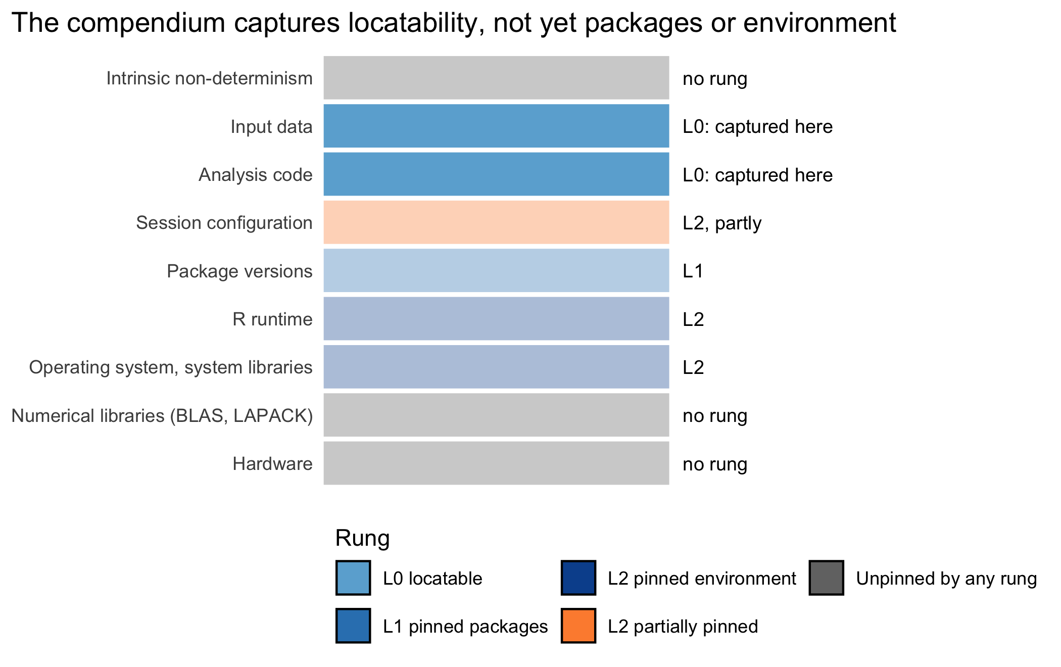
The purpose of this article is to show how the R package can be a suitable template for organising files into a research compendium to enhance the reproducibility of research.
Marwick, Boettiger, and Mullen, Packaging Data Analytical Work Reproducibly Using R (and Friends) (2018)
By the end of this chapter you will be able to look at a folder of scripts and spreadsheets and name what kind of research object it is trying to be. You will also be able to draw the line between what counts as raw input and what counts as a derived product. Finally, you will be able to say exactly which single build gate, R CMD check, a tidy directory earns for free, and what that gate still leaves unexamined.
We begin by placing the chapter on the determinant stack of Chapter 3. In the sense of pinning a package version or a system library, this chapter captures nothing on that stack. What it captures are the two layers that sit above the packages and the system, the analysis code and the input data, by making them locatable and organized in the first place. Figure 5.1 marks these two layers. A compendium is what first turns a scatter of files into something a reader can find and name, and within which the reader can locate the raw-versus-derived boundary. This is the L0 rung and no further.
plot_determinant_stack(
captures = c('Analysis code', 'Input data'),
title = 'The compendium captures locatability, not yet packages or environment')Consider a first-year epidemiology student who has spent three months on a cohort analysis. The analysis is an incident-diabetes study drawn from a registry, with a cleaning script, a handful of models, four figures, and a draft of a results section. The work exists, but it exists as a scatter. The cleaning script sits in a downloads folder, and the models sit in a second file that reads a spreadsheet whose path is hard-coded to one laptop. The figures are loose png files pasted by hand into a manuscript, and the record of which package versions produced any of it is nowhere at all. Nothing here is wrong as statistics. The difficulty is that the analysis is not an object. It cannot be handed to a colleague, cited, archived, or re-run, because there is no single thing to hand over.
The remedy is to make the analysis one object. A research compendium is that object. It is a single, self-describing directory that bundles the code, the data, the prose, and the record of the environment in which the analysis was run. Its contents are organized by convention, so that another person, or the same person a year later, can find every part and regenerate the result. The compendium is the third of the recurring ideas of this book, after the levels ladder and the capture-versus-validate distinction. It is also the one that gives the other two something to act on. A reproducibility level is a property of a compendium; a validation gate is a check run against a compendium.
The compendium also sets the starting rung on the ladder. Merely by being a version-controlled directory whose parts can be located, a compendium reaches L0, locatable. It is not yet L1, because nothing has pinned the package versions. It is not yet L2, because nothing has pinned the environment. And it is certainly not yet L3, because nothing has re-run it and shown the numbers to match a recorded baseline. The compendium provides the container into which the later chapters install those higher guarantees.
The remainder of the chapter proceeds as follows. The three judgments that remain the analyst’s alone come first, and we then trace where the idea of the compendium comes from and why the R package became its container. We next set out the Five Pillars and the directory layout, then the README, the data dictionary, and project-oriented paths with here. The five archetypes follow, each with a health-sciences example and a note of how it weighs the chapters ahead. Lastly, we consider progressive disclosure, work one compendium through two archetypes, and measure this book’s own compendium against the Five Pillars.
Three judgments at the center of this chapter are the analyst’s alone. No tool scaffolds them. Getting them wrong produces a tidy directory that is nonetheless the wrong shape for the work.
Naming the archetype. The analyst must decide what kind of object the project is: a data analysis, a manuscript, a reusable package, a simulation study, or a blog. This choice governs the layout, whether a report is rendered, and which gates apply. It is a statement of intent, not a technical setting, and it is the organizing decision of the chapter.
Fixing the raw-and-derived boundary. The analyst must decide what is an immutable input and what is a product of the analysis. A file placed in raw_data/ is a promise that it will never be modified; a file in derived_data/ is a promise that it can always be regenerated from the raw inputs and the code. No program can draw this line, because it depends on where the analyst judges the science to begin.
Deciding what becomes a function. The analyst must decide which code is a throwaway pipeline step, belonging in analysis/scripts/, and which is a reusable procedure worth documenting and testing, belonging in R/. This judgment determines what R CMD check and the test suite will actually protect, and it is revisited continuously as a project matures.
DESCRIPTION, NAMESPACE, an R/ directory) that makes a directory a valid R package, and therefore checkable by the R build tools.R CMD check. The standard R command that builds a package, runs its tests, and applies dozens of standardized checks; here it is a universal integrity gate on the compendium’s package skin (R/, the tests, DESCRIPTION). It does not check analysis/, which the build excludes.Dockerfile, renv.lock, .Rprofile, the source code, and the data.We turn now to the history of the idea, which is older than its tooling and which explains the shape of the modern object. Gentleman and Temple Lang, writing in 2007, proposed the compendium in its current sense: a document that combines text, code, and data in a form a reader can actually execute, rather than a paper that merely describes an analysis performed elsewhere (Gentleman & Temple Lang, 2007). The proposal drew on Knuth’s earlier notion of literate programming, in which prose and code are woven into one source (Knuth, 1984). For some years the compendium remained an aspiration without a conventional implementation. Peng, arguing that reproducibility should be treated as a minimum standard for computational science, sharpened the motivation without settling the container (Peng, 2011).
The decisive move came from Marwick, Boettiger, and Mullen. They observed that a container of exactly the required shape already existed and was in daily use by thousands of R developers: the R package (Marwick et al., 2018). An R package, as standardized by Wickham (Wickham, 2015), already provides a DESCRIPTION file recording metadata and dependencies and an R/ directory for reusable functions. It also provides a tests/ directory for unit tests, a vignettes/ directory for long-form prose, and a rigorously specified build system. Marwick and colleagues extended this layout with a single top-level analysis/ directory holding subdirectories for raw data, derived data, scripts, figures, and the manuscript itself. They packaged the whole as the rrtools tool. The resulting compendium can be installed, tested, and checked with the very same commands used for any R package. Nüst, Boettiger, and Marwick later wrote a companion guide on how to read such a compendium. That such a guide exists is a useful sign that the object had matured enough to have a reading protocol at all (Nüst et al., 2018).
The choice of the R package as the container is the most consequential design decision in this lineage. At first it looks like a convenience, the reuse of a familiar layout. However, it also makes an existing, rigorous, and universal gate apply to the compendium’s package skin for free. In this section we state both what that gate reaches and what it does not.
The gate is R CMD check. When R was designed as a system for distributing statistical software, its authors built a command that takes a package and subjects it to dozens of standardized checks. The command checks that the code parses and loads, that every documented function matches its documentation, and that declared dependencies are actually available. It also checks that the examples run and that the tests pass. The command was built to keep the tens of thousands of packages on CRAN mutually consistent. By dressing a compendium in the R-package skin, we inherit this entire apparatus at no cost. A compendium that passes R CMD check is one whose functions in R/ load, whose stated dependencies resolve, and whose tests succeed. These properties hold in a clean process that carries none of the author’s accumulated and undeclared state.
The qualification ‘in R/’ is exact, not cautious. But what, precisely, does the check examine? As rcmdcheck::rcmdcheck() and devtools::check() run it, R CMD check does not check the directory it is pointed at. It checks the package tarball that R CMD build makes from that directory, and the build omits every path listed in .Rbuildignore. (Plain R CMD check on a directory skips the build, but it parses R code only in the package’s own directories, such as R/ and tests/, so the scripts in analysis/ go unparsed either way.) A compendium lists ^analysis$ there, as it must, because raw data, derived files, and a manuscript do not belong in an installable package. The consequence is that the check never sees analysis/. An analysis script with a syntax error, or one that calls library() on a package declared nowhere, passes R CMD check with no error, warning, or note. The same undeclared package used inside a function in R/ draws a WARNING (‘:: or ::: import not declared from’). The code in analysis/ therefore needs gates of its own. These are a render gate, which executes it, and a dependency scan, which reads it for packages that the lockfile does not pin. Both are developed in Chapter 12.
A new compendium that omits ^analysis$ from .Rbuildignore, or deletes the line while editing the file by hand, does not fail silently. R CMD build then tries to fold the raw data, the derived files, and the rendered report into the installable tarball. This can make the build slow or bloat the package beyond what CRAN or a reviewer will tolerate. It can also fail outright on a binary data file the build process cannot parse as package data. The fix is to treat .Rbuildignore as part of the package skin, checked into version control like DESCRIPTION, not as an incidental dotfile.
The R-package structure is therefore part of what makes a directory a compendium. Every archetype we shall meet below, however different in outward shape, carries the same minimal R-package skin. It follows that R CMD check is the one gate that applies to all of them. A manuscript compendium adds a render gate on top; a simulation compendium adds a seeding discipline; a package compendium leans on the check most heavily of all; but the universal floor is the same. It is, however, a floor under R/ and the tests, not under the analysis. This is one reason the analyst’s third judgment, what becomes a function, matters: code moved into R/ comes under the check, and code left in analysis/ does not. We return to this point when we tabulate the archetypes, because it is the thread that unifies them.
The R-package skin need not be written by hand. Two packages automate it: usethis writes the files of the skin, and devtools runs the development loop on top of them. The chunk below lists the commands a compendium needs, in the order a new project meets them.
lock <- jsonlite::read_json('../../renv.lock')
lock_pkgs <- names(lock$Packages)
skeleton_tools <- c('usethis', 'devtools', 'pkgdown',
                    'pkgload', 'tinytest')
in_lock <- skeleton_tools %in% lock_pkgs
names(in_lock) <- skeleton_tools
in_lock
#>  usethis devtools  pkgdown  pkgload tinytest
#>    FALSE    FALSE    FALSE     TRUE     TRUE
# Not run here: several of these packages are outside
# renv.lock (see the text).
usethis::create_package('cohortstudy')
usethis::use_r('cohort')
usethis::use_gpl_license(version = 3)
usethis::use_package('survival')
tinytest::setup_tinytest('.')
usethis::use_pkgdown()
devtools::load_all()
devtools::document()
devtools::check()
pkgdown::build_site()We do not run the second chunk. Of the five tools it calls, usethis, devtools and pkgdown are not recorded in this repository’s renv.lock, so running them would step outside the pinned library; only pkgload and tinytest are recorded. That absence is defensible for development tools, since what they produce (DESCRIPTION, NAMESPACE, the help files in man/) is committed. A reproducer uses those files without rerunning the tools, and can run R CMD check from the shell with none of them installed.
The first six calls run once, or once per new file. create_package() writes DESCRIPTION, NAMESPACE, and R/, the minimal skin of the previous section. use_r() creates or opens a file in R/, the place where a function comes under the check. The license call writes the License field and a license file. This compendium’s DESCRIPTION records GPL-3. The call that writes GPL-3 is use_gpl_license(version = 3); others, such as use_mit_license() or use_cc0_license(), write other licenses, and the choice is argued in Chapter 13. use_package() adds a package to Imports, which is how the undeclared-import WARNING of the previous section is cleared. Because the book tests with tinytest (Loo, 2020), its setup_tinytest() takes the place of the use_testthat() most tutorials show. It creates inst/tinytest/ and the runner tests/tinytest.R, and adds tinytest to Suggests, where this compendium’s DESCRIPTION has tinytest (>= 1.4.0).
The next three calls form the loop that is repeated while the code in R/ changes. load_all() makes the package’s functions available in the session by simulating a build, an install, and an attach, and Wickham & Bryan (2023) recommend it over source() for package work. It is supplied by pkgload, which this chapter’s own first chunk calls directly. document() turns the roxygen comments above each function into help files and regenerates NAMESPACE. check() builds the tarball and runs R CMD check on it, the gate of the previous section, with the same blind spot for analysis/. A useful habit is to run check() before any commit that touches R/, DESCRIPTION, or the tests.
pkgdown builds a website from the help files, the README, and any vignettes. use_pkgdown() runs once and writes _pkgdown.yml; build_site() is rerun to refresh the site. A site is documentation, not a gate. It earns its place in the R-package archetype, whose users read reference pages, and is seldom worth maintaining for a data analysis. The full treatment of each step, and of the many usethis helpers not shown, is R Packages (2e) by Wickham and Bryan (Wickham & Bryan, 2023). Its chapter ‘The Whole Game’ runs the loop end to end on a toy package, its ‘Website’ chapter covers pkgdown, and an appendix treats R CMD check in detail.
Having settled the container, we turn to what it holds. A compendium is defined by convention, but it manages a specific and small set of artifacts. The zzcollab framework organizes these as the Five Pillars. These are the five things a compendium reads, writes, and version-controls, one for each point at which reproducibility can be captured (team, 2026). An analysis is reproducible only to the extent that all five are captured. Moreover, the pillars are layered rather than independent, each resting on the ones beneath it.
Computational environment, captured by the Dockerfile. This pillar fixes the operating system, the R version itself, the system libraries, and the document toolchain, all the software beneath the R packages. It is the subject of Chapter 7.
Package versions, captured by renv.lock. This pillar records the exact version of every R package the analysis loads, so that the same set can be restored on another machine. It is the subject of Chapter 6.
Session configuration, captured by the project .Rprofile. This pillar fixes the R options, the locale and timezone, and the thread counts that shape a session before any user code runs. A profile can also override the random-number-generator kind, but such an override is secured only by an explicit RNGkind() call in the analysis code, and the seed belongs there too (Chapter 3, Chapter 11).
Source code, captured by the version-control history. This pillar holds the scripts, the functions, the manuscript source, and the tests that implement the analysis.
Data, captured either by inclusion in the compendium, for small redistributable files, or by reference to an external repository with a resolvable identifier, for large or restricted data.
Two of the pillars are not coordinate with the other three. Source code and data, pillars four and five, are the inputs whose re-execution is the goal. The environment, packages, and session, pillars one through three, are the conditions under which that re-execution occurs. This chapter is about the container that holds all five and the shape that container takes. The individual pillars are developed in the chapters named against them.
This chapter’s own practice stops at naming and separating the five artifacts. It leaves their actual capture, and the rung that capture buys, to the chapters named against each pillar above.
We now make the layout concrete. The following is the top-level structure of a zzcollab compendium. The block is illustrative and is not executed.
penguin-analysis/
├── DESCRIPTION           # package metadata and dependencies
├── NAMESPACE             # generated; exported functions
├── LICENSE
├── R/                    # reusable, documented functions
├── man/                  # generated function documentation
├── tests/                # tinytest runner
├── inst/tinytest/        # unit tests (test-*.R)
├── vignettes/            # long-form prose
├── analysis/
│   ├── data/
│   │   ├── raw_data/       # immutable inputs
│   │   ├── derived_data/   # regenerable script outputs
│   │   └── metadata/       # data dictionaries, provenance
│   ├── scripts/           # numbered pipeline steps
│   ├── report/            # report.Rmd / index.qmd manuscript
│   ├── figures/           # generated figures
│   └── tables/            # generated tables
├── Dockerfile            # Pillar 1: environment
├── renv.lock             # Pillar 2: package versions
├── .Rprofile             # Pillar 3: session configuration
├── Makefile              # workflow entry points
├── zzcollab.yaml         # configuration: base image, archetype
├── .zzcollab-state       # generated state record; never hand-edited
└── .github/workflows/    # continuous-integration definitions
Above the analysis/ directory sits the standard R-package machinery, and this is the skin that makes R CMD check apply. Within analysis/ sits the research proper, in the Marwick convention. Its raw-and-derived data separation is the analyst’s second judgment made physical. At the root sit the three environment artifacts, one per pillar. Alongside them sit the Makefile that provides the commands and the zzcollab.yaml that records, among a small set of parameters, the archetype. That last file is our bridge to the centerpiece of the chapter. The archetype is a first-class parameter recorded there, elicited at creation time alongside the choice of base image.
The directory listing above names a README nowhere, and that absence is not an oversight to copy. A compendium that captures all five pillars perfectly but ships without a README still fails the first test a stranger applies to it, because the stranger has no entry point. The NHS RAP Community of Practice makes a README one of the criteria of its baseline level, alongside code in an open-source language, version control, peer review of the code, and open publication. A repository meets the README criterion only once it ‘includes a README.md file (or equivalent) that clearly details steps a user must follow to reproduce the code’ (NHS England RAP Community of Practice, 2024). A README.md at the project root should state, in order, what the project is for, how to reproduce it, and where the data dictionary lives for anyone who needs the columns rather than the narrative. The reproduction instructions name the make target or Rscript command that runs the pipeline end to end, and the archetype-specific gate from Chapter 3 that passing it claims.
The data dictionary is a second, separate document, usually in analysis/data/metadata/ or beside the extract it describes. It answers a question the README should not try to: what is each column, exactly. At minimum it gives, per column, the name, its type, a one-line meaning, its units where numeric, and its provenance. Provenance here means whether the column was measured, derived, or simulated and by what script. This book’s own analysis/data/README.md is a worked, if unusually candid, example. Because the extract it describes is synthetic, the dictionary can also say outright which rows are planted defects and why. A real data use agreement would instead replace that disclosure with an access-control statement. The columns table there (mrn, patient_name, hba1c, and seven more, each with a type and a one-line meaning) is the shape to imitate. On the other hand, the provenance section above it, naming the exact generator script and seed, is the part a real project cannot write the same way. A real extract’s provenance is the originating system and the extraction date, not a committed script.
A README that names the command still leaves a reproducer guessing what the command needs. The template README of the Social Science Data Editors, written for replication packages, gives this a section of its own, ‘Computational requirements’ (Vilhuber et al., 2022). Adapted to an R compendium, that section asks for the first four items below, and the template’s ‘List of tables and programs’ supplies the fifth.
renv.lock, and names the image digest once there is one.This book’s cohort compendium makes a compact example. Its repository does not yet have a README.md at the root, so the excerpt below is the section such a file would carry. Every value in it, from the R version to the seed’s line number and the runtime, is read from the repository or measured when this chapter is rendered, which is the same rule the README itself should follow.
## Computational requirements

- Software: R 4.6.1, packages as in renv.lock
  (restore with renv::restore()); key packages
  survival 3.8-6, withr 3.0.3, tinytest 1.4.3.
- Randomness: simulate_cohort.R calls
  set.seed(20260908) once, at line 19;
  bootstrap_cox_ci() sets seed 20260908 (B = 1000)
  with withr::with_seed(). Sampler kinds:
  Mersenne-Twister, Inversion, Rejection.
- Runtime: 3.1 s for the analysis and bootstrap
  (under 10 min).
- Hardware: aarch64-apple-darwin23, 8 logical cores.

| Output                 | Produced by |
|------------------------|-------------|
| Synthetic extract      | analysis/scripts/simulate_cohort.R |
| Cox HR for BMI, 95% CI | R/cohort.R: run_canonical_analysis() |
| Bootstrap interval     | R/cohort.R: bootstrap_cox_ci() |
| Recorded baseline      | analysis/scripts/generate_baseline.R |
| Baseline check (L3)    | inst/tinytest/test-baseline-cohort.R |
Two points in the excerpt are easy to miss. The extract and the bootstrap draw from separate seeds, and the README says where each is set, because a reader who finds only one may assume the other draws from the clock. The runtime and hardware are those of the machine that last rendered this chapter, not of the reader’s; they tell a reproducer whether a run is expected to take seconds or days, not what their own run will take. The excerpt also omits memory, which base R does not report in a portable way; an author measures it and adds the figure by hand.
here, not setwd()
A script that opens with setwd('/Users/jane/project') reproduces on exactly one machine: Jane’s. The fix taught by the here package is to mark the project root once, with a file such as .here or the marker RStudio and Git already leave behind. Every path is then built with here::here(), which walks up from the working directory until it finds that marker and returns paths relative to it from there on (Bryan & Hester, 2024). Consider a script that reads here::here('analysis', 'data', 'raw_data', 'cohort_raw.csv'). It resolves the same file whether R is launched from the project root, from analysis/report/, or from a continuous-integration runner that checks the repository out to a different absolute path each time. This holds because the path is computed from the marker rather than typed as a string.
This book’s own chapters, inspected directly, show why the discipline matters even without setwd(). Several chapters reach the cohort extract with '../data/raw_data/...'. However, 08-testing-quality.qmd reaches the same file with '../../analysis/data/raw_data/...', which climbs to the project root and back down again. From analysis/report/ the two strings name one file by different routes, and nothing but the author’s care keeps the two forms in agreement. Every one of these paths works only because the author tracked, chunk by chunk, how many ../ steps the renderer’s working directory is from the target file. By contrast, here::here('analysis', 'data', 'raw_data', 'cohort_raw.csv') would resolve identically from any of these chunks, because it does not depend on the renderer’s starting point at all. The relative-path convention is not wrong, exactly. It is fragile in a way that is invisible until a chunk is moved, copied into a different chapter, or run from a different tool.
We come now to the centerpiece of the chapter. In this section we make the point this book returns to in every chapter: a research compendium need not be a manuscript. Once we have seen the analysis/report/ directory, it is easy to assume that a compendium always exists to render a paper. That is the common case, but it is one case among five.
zzcollab treats the research archetype as a first-class initialization parameter, orthogonal to the choice of computational environment (team, 2026). Where the base image fixes the environment, the archetype determines the starting scaffolding: the directory emphasis, whether a primary report exists, and which validation gates apply on top of the universal one. Five archetypes are advertised. Because every one of them carries the minimal R-package skin, R CMD check remains the universal gate across all five. The framework’s own whitepaper stresses this point in its account of the archetype axis. The reproducibility machinery is identical; what varies is the shape of the work and the gates it warrants. We take each in turn, with a health-sciences example, and then tabulate the differences.
The first archetype is the exploratory and confirmatory data analysis with no manuscript as its primary organizing document. This is the closest to the original rrtools use case, and it is the archetype of the epidemiology student of our orientation. The work lives in analysis/scripts/, as numbered pipeline steps, and in analysis/figures/, with the derived datasets in analysis/data/derived_data/. Consider an incident-diabetes cohort study. A cleaning script reads the registry extract from raw_data/ and writes an analysis-ready table to derived_data/. A modeling script fits a Cox proportional-hazards model and writes the coefficient table to tables/, and a plotting script writes the Kaplan-Meier curves to figures/. There may be a short results document, but the deliverable is the pipeline and its outputs.
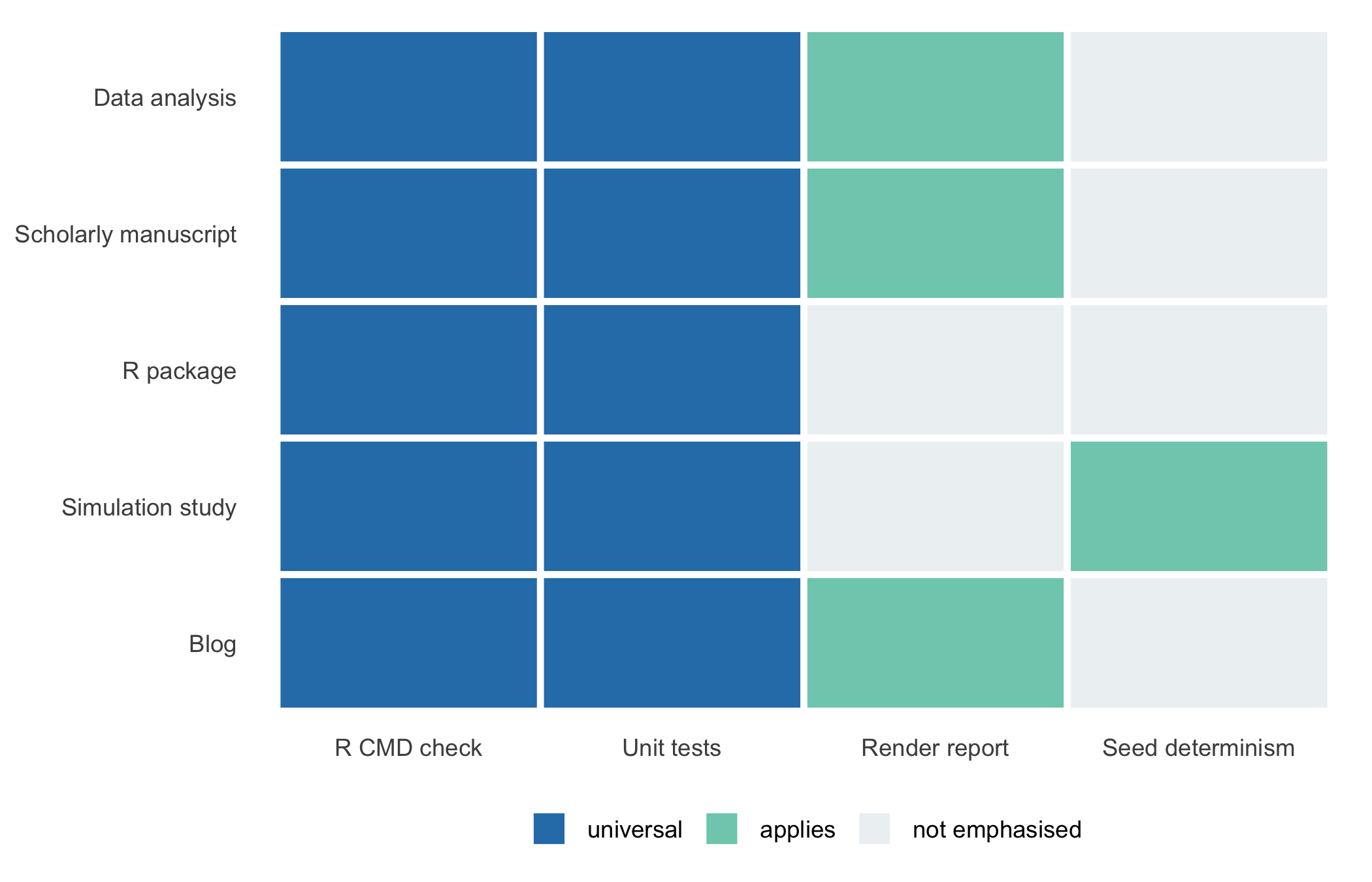
The applicable gates are the universal R CMD check and the unit tests. The latter guard the cleaning logic and the data invariants. For example, they check that the cohort has the expected number of subjects. They also check that a derived rate matches a value recorded in a baseline file within a stated tolerance, rather than merely falling in a plausible range. A render gate is optional here, because there may be no report to render. The reproducibility machinery, environment and packages and session, is nonetheless present in full.
The second archetype makes the manuscript the organizing principle. A report.Rmd or index.qmd file in analysis/report/ is created on day one and written in parallel with the analysis, so that the prose and the numbers never drift apart. Every figure in the paper is regenerated on each render, rather than pasted in by hand. A representative deployment is a study of the comorbidity of PTSD, depression, and diabetes among Black women drawn from a trauma-study cohort. The study uses variable selection, multiple imputation, and causal mediation analysis. The compendium organizes the manuscript in analysis/report/report.Rmd, the statistical functions in R/ with roxygen2 documentation, the analysis pipeline in analysis/scripts/, and the imputed datasets in analysis/data/derived_data/.
Here the render gate is central, not optional. A validation run rebuilds the report from source, and a failure to render is a failure of the compendium. The gates are therefore R CMD check, the unit tests, and the render of report.Rmd to PDF. This is the archetype most readers imagine when they hear the word compendium, and it is only the second of five.
The third archetype arises when the reusable code matures into something of general interest. At that point R/, man/, and tests/ become the first-class content, and the compendium is shareable as a CRAN-style package. What distinguishes this archetype is that there is no report to render at all. A package that generates publication-quality clinical-trial summary tables has no manuscript as its deliverable; its deliverable is the exported, documented, tested function. A representative deployment is exactly such a summary-table package, hosting its source in R/, its examples in vignettes/, and its documentation as a generated website.
The gates for this archetype are R CMD check, run at its full strength, and the unit tests. There is no render gate, because there is nothing to render. This case is the clearest refutation of the manuscript-only view. An entirely valid, fully reproducible compendium can produce no report whatsoever, and its integrity rests on the universal check and the tests alone.
The fourth archetype is the simulation study, such as a power calculation or an assessment of the operating characteristics of a proposed trial design. In such a study the compendium enumerates a grid of parameter configurations, runs Monte Carlo replicates at each, and stores the results. The layout leans on analysis/scripts/ for the simulation driver and on analysis/data/derived_data/ for the stored replicate results. These are treated as derived data because they can be regenerated from the code and the seeds.
But what makes a simulation reproducible at all? The distinguishing discipline of this archetype is seeding. A simulation whose random draws are not pinned by an explicit set.seed() is not reproducible even in principle, because a second run produces different numbers by construction. The archetype therefore emphasizes explicit seeding and parallel execution. A recommended practice is to store a seed column alongside the parameter grid so that each replicate is individually reproducible. Consider a power simulation for a longitudinal trial. The driver builds a grid over sample size and effect size and assigns each row an integer seed. It then simulates a dataset for each row, fits the planned model, and records whether the null was rejected. The empirical power is then the rejection rate within each cell. The gates are R CMD check, the unit tests, and, as an emphasis particular to this archetype, a baseline test that compares the seeded output with a value recorded in an earlier session and committed (Chapter 11). A second call in the same session is not such a test, because it agrees with the first even when the generator has changed. A render gate is optional, since the deliverable is often the stored results rather than a paper.
The fifth archetype is the blog or lab notebook, in which the compendium renders, in the general case, not one report but many documents. A teaching blog carrying a series of methods posts, or a running lab notebook of analyses, is a single compendium. Its analysis/ tree may hold many index.qmd files, each rendered to a static site by the same machinery that renders a manuscript. The framework’s representative deployment is the limiting case of a single post. Integration with Quarto (Allaire et al., 2024) enables publication to the site from the same compendium that produced the underlying analyses. As a result, the full five-pillar reproducibility stack applies to web-published teaching content without any change to the workflow.
The gate here is again the universal R CMD check, joined by a render gate that must succeed for each post the compendium carries. The multiplicity is the distinguishing feature of the general case. That is, a blog compendium is a render-many, where the manuscript is a render-one and the package is a render-none.
The five archetypes and their differences are summarized in Table 5.1, and Figure 5.2 shows which validation gates apply to each. Both are best read across the rows, to see how the layout and the gates vary, and down the two universal columns, to see how much stays fixed.
library(tibble)
library(knitr)

archetypes <- tibble::tibble(
  archetype = c(
    'Data analysis', 'Scholarly manuscript', 'R package',
    'Simulation study', 'Blog'
  ),
  directory = c(
    'analysis/scripts/, analysis/figures/',
    'analysis/report/',
    'R/, man/, tests/',
    'analysis/scripts/, derived_data/',
    'many analysis/ index.qmd posts'
  ),
  report = c(
    'Optional', 'Yes, to PDF', 'No',
    'Optional', 'Yes, many'
  ),
  gate = c(
    'R CMD check and tests',
    'R CMD check plus render',
    'R CMD check and unit tests',
    'R CMD check plus seed determinism',
    'R CMD check plus render of each post'
  ),
  example = c(
    'Incident-diabetes cohort analysis',
    'PTSD and diabetes comorbidity paper',
    'Clinical-trial summary-table package',
    'Power and operating-characteristics simulation',
    'Teaching blog or lab notebook'
  )
)

knitr::kable(
  archetypes,
  col.names = c(
    'Archetype', 'Directory emphasis', 'Renders a report?',
    'Primary validation gate', 'Health-sciences example'
  )
)| Archetype | Directory emphasis | Renders a report? | Primary validation gate | Health-sciences example |
|---|---|---|---|---|
| Data analysis | analysis/scripts/, analysis/figures/ | Optional | R CMD check and tests | Incident-diabetes cohort analysis |
| Scholarly manuscript | analysis/report/ | Yes, to PDF | R CMD check plus render | PTSD and diabetes comorbidity paper |
| R package | R/, man/, tests/ | No | R CMD check and unit tests | Clinical-trial summary-table package |
| Simulation study | analysis/scripts/, derived_data/ | Optional | R CMD check plus seed determinism | Power and operating-characteristics simulation |
| Blog | many analysis/ index.qmd posts | Yes, many | R CMD check plus render of each post | Teaching blog or lab notebook |
library(ggplot2)

archs <- c(
  'Data analysis', 'Scholarly manuscript', 'R package',
  'Simulation study', 'Blog'
)
gates <- c(
  'R CMD check', 'Unit tests', 'Render report',
  'Seed determinism'
)
grid <- expand.grid(
  archetype = archs, gate = gates,
  stringsAsFactors = FALSE
)

renders <- c('Scholarly manuscript', 'Blog')
seeded <- c('Simulation study')

grid$status <- 'not emphasised'
grid$status[grid$gate %in% c('R CMD check', 'Unit tests')] <-
  'universal'
grid$status[grid$gate == 'Render report' &
              grid$archetype %in% renders] <- 'applies'
grid$status[grid$gate == 'Seed determinism' &
              grid$archetype %in% seeded] <- 'applies'

grid$archetype <- factor(grid$archetype, levels = rev(archs))
grid$gate <- factor(grid$gate, levels = gates)
grid$status <- factor(
  grid$status,
  levels = c('universal', 'applies', 'not emphasised')
)

# Non-color cue: a point shape per status, so universal and
# selective cells differ by shape as well as hue (WCAG 1.4.1).
# The two fills are only 1.34:1 apart, so the shape carries the
# distinction; the white markers are 7.1:1 and 5.3:1 against them.
# Point shapes rather than a text glyph, because the PDF device
# cannot encode a Unicode circle. The shape scale shares the fill
# scale's labels so the two merge into one legend, and a reader who
# cannot separate the hues can still read the key by shape.
marked <- grid[grid$status != 'not emphasised', ]
status_labels <- c(
  'universal'      = 'Universal',
  'applies'        = 'Selective',
  'not emphasised' = 'Does not apply'
)

ggplot(grid, aes(x = gate, y = archetype, fill = status)) +
  geom_tile(colour = 'white', linewidth = 1.2) +
  geom_point(data = marked, aes(shape = status), colour = 'white',
             size = 3.5) +
  scale_shape_manual(
    values = c('universal' = 16, 'applies' = 17,
               'not emphasised' = NA),
    labels = status_labels, drop = FALSE
  ) +
  scale_fill_manual(
    values = c(
      'universal'      = '#1a5c8c',
      'applies'        = '#1e7a50',
      'not emphasised' = '#7a8a9c'
    ),
    labels = status_labels
  ) +
  guides(fill = guide_legend(override.aes = list(size = 2.5))) +
  labs(x = NULL, y = NULL, fill = NULL, shape = NULL) +
  theme_minimal(base_size = 11) +
  theme(
    panel.grid = element_blank(),
    legend.position = 'bottom'
  )
The reproducibility machinery is identical across the five archetypes; only its weight shifts. Table 5.2 is the reference every later chapter points back to rather than restates. For each archetype, it records how the ladder reads it (Chapter 3) and how heavily it leans on a sealed render (Chapter 9). It also records which kind of test carries its weight (Chapter 11) and how its continuous-integration gates are configured (Chapter 12). Lastly, it records how much a pipeline tool earns its keep (Chapter 10) and how the compendium is ultimately shared (Chapter 13).
| Archetype | Ladder (Chapter 3) | Literate programming (Chapter 9) | Testing (Chapter 11) | CI gates (Chapter 12) | Pipeline (Chapter 10) | Sharing (Chapter 13) |
|---|---|---|---|---|---|---|
| Data analysis | Same rungs as a manuscript; L3 via a baseline on a derived rate | Light; an internal HTML summary, not a typeset report | Leans on data-validation and reproducibility tests | Render gate only if a report exists | Strong case for targets, since it is re-run constantly and skipping unchanged steps saves time |
Deposited as itself |
| Scholarly manuscript | Full apparatus; L3 compares tables and figures with recorded baselines | Center of gravity; the sealed render this chapter is built around | Adds a report-renders-and-matches-baseline test | Render gate is central, not optional | Modest; often a one-target build around the sealed report | Deposited beside the article it supports |
| R package | L1 and L2 as for any archetype, since R CMD check is a gate, not a rung; L3 via a baseline on function output after a clean rebuild |
Largely absent; help pages and vignettes stand in | Native home of unit testing; R CMD check runs the suite |
No render gate unless a vignette exists | None; R CMD check plays the corresponding role |
Also released to CRAN or an R-universe, not only archived |
| Simulation study | L2 is nominal without the seed discipline; RNG kind is the load-bearing determinant | Thin; a presentation layer over pre-computed, stored results | Leans hardest on the seed-determinism test | A reduced, fixed-seed grid runs under CI; the full grid runs elsewhere | Strongest case of the five; targets branching maps the parameter grid |
Recorded seeds and the union lockfile are what a re-runner needs |
| Blog | Applies post by post; L3 needs a baseline per post | Central but multiplied across many rendered posts | Tests the code each post’s examples depend on | Render gate iterates over every post | Rebuilds only the posts whose sources changed | Deployed as a website; the compendium behind it is still deposited |
But must a project choose one archetype and keep it? The five archetypes can also be stages a single project passes through. The framework’s most useful structural property is that the same layout supports the whole trajectory without reorganization. This is what the framework calls progressive disclosure: the same directory layout, the same Makefile, and the same Five Pillars carry a project from one archetype to the next.
The trajectory is easy to picture, and it is the one our epidemiology student is likely to walk. The project begins as a data analysis: scripts and figures, no manuscript. As the findings firm up, a report.Rmd is added to analysis/report/ and the project becomes a manuscript compendium, with the render gate now active. Nothing already written needs to move. In the course of the analysis a cleaning routine and a modeling helper prove useful enough to document and test, so they migrate from analysis/scripts/ into R/. The package archetype’s gates begin to bite on them without any change to the layout. Should one of those functions reach general interest, the compendium can be shared as a package, with its R/ and man/ and tests/ now first-class. The analysis/ directory then recedes to a development notebook. The same compendium has been, in turn, a data analysis, a manuscript, and a package, and at no point was it reorganized.
The archetype therefore describes a project’s current emphasis; it is not a permanent category. The reproducibility machinery is invariant across the archetypes and across the transitions between them. It is this invariance that lets a project evolve without leaving the reproducible state it started in. The worked example that follows traces the first part of this trajectory in detail.
To make the progressive-disclosure trajectory concrete, we follow a single compendium through its first two archetypes. We stay at the level of the directory and the gates rather than the analysis. Suppose our student begins the incident-diabetes study. The compendium is created and its archetype recorded as a data analysis. The shell session below is illustrative and is not executed.
$ mkdir diabetes-cohort && cd diabetes-cohort
$ zzc analysis  # tidyverse base-image profile; archetype set separately
The student places the registry extract under raw_data/ and writes analysis/scripts/01_clean.R to produce a derived cohort table. The student then writes analysis/scripts/02_model.R to fit the Cox model. A unit test in inst/tinytest/ asserts the cohort size and that the fitted hazard ratio matches a value recorded in a committed baseline file, within a stated tolerance. This is a test that can actually fail if the model’s inputs or the survival version drift. By contrast, a bound such as ‘no hazard ratio is negative’ would be satisfied by every correct and every broken fit alike. At this point the only gates that apply are the universal check and the tests, run in a clean environment:
$ make check-renv     # dependencies declared and locked
$ make docker-test    # tinytest only
$ make docker-check   # R CMD check
Some weeks later the results are firm enough to write up. The student adds analysis/report/report.Rmd, moving the figure code out of 02_model.R and into report chunks that regenerate the figures on render. The compendium is now a manuscript, and the archetype line in zzcollab.yaml is updated to reflect it. However, not a single existing file has moved. A render gate now joins the others:
$ make docker-render # rebuild report.Rmd to PDFThe cleaning routine, meanwhile, has grown into a general helper worth documenting. It therefore migrates from analysis/scripts/01_clean.R into R/prepare_cohort.R, gains a roxygen2 block, and picks up its own unit tests. The package archetype’s discipline now protects it, and R CMD check verifies that the documentation matches the function signature. The same compendium is now doing the work of three archetypes at once, on one unchanged layout. Each gate applies to the part of the project that warrants it.
The examples so far have all described a hypothetical student’s compendium. We now perform the same classification exercise on this book’s own running cohort compendium, as it sits in this repository when the chapter is rendered.
raw <- load_cohort('../data/raw_data/cohort_raw.csv')
cohort <- clean_cohort(raw)
pillars <- c(
  environment_dockerfile = file.exists('../../Dockerfile'),
  packages_renv_lock = file.exists('../../renv.lock'),
  session_rprofile = file.exists('../../.Rprofile'),
  source_code_r_cohort = file.exists('../../R/cohort.R'),
  data_generator = file.exists('../scripts/simulate_cohort.R')
)
pillars
#> environment_dockerfile     packages_renv_lock       session_rprofile
#>                  FALSE                   TRUE                   TRUE
#>   source_code_r_cohort         data_generator
#>                   TRUE                   TRUE
sum(pillars)
#> [1] 4
nrow(raw)
#> [1] 338
nrow(cohort)
#> [1] 337
pillar_label <- c(
  environment_dockerfile = 'the environment pillar (`Dockerfile`)',
  packages_renv_lock = 'the package-versions pillar (`renv.lock`)',
  session_rprofile = 'the session pillar (`.Rprofile`)',
  source_code_r_cohort = 'the source-code pillar (`R/cohort.R`)',
  data_generator = 'the data pillar (`simulate_cohort.R`)'
)
pillars_absent <- if (any(!pillars)) {
  paste(pillar_label[!pillars], collapse = ' and ')
} else {
  'no pillar'
}
rung <- if (pillars[['packages_renv_lock']] &&
              pillars[['environment_dockerfile']]) {
  'L2'
} else if (pillars[['packages_renv_lock']]) {
  'L1'
} else {
  'L0'
}
In this repository, 4 of the Five Pillars have an artifact. The source-code pillar is R/cohort.R, under version control. The data pillar is the committed generator analysis/scripts/simulate_cohort.R, which writes the synthetic extract from a fixed seed; the CSV it writes is gitignored, so the chunk checks the generator, not the extract. Of the five, the compendium still lacks the environment pillar (Dockerfile). Against the archetype table above, this compendium is a data analysis. Its deliverable is the pipeline of R/cohort.R and the chunks this book’s chapters run against it, not a rendered manuscript of its own. The applicable gates are therefore the universal R CMD check and the unit tests, with no render gate required. Measured against the Five Pillars, the compendium is at L1, the rung Chapter 3 computes for it from the same files. The lockfile entry, TRUE, and the Dockerfile entry, FALSE, decide the rung. The source-code and data pillars make a compendium locatable, and the session pillar fixes the options a session starts with, but none of the three pins a package version or an environment.
A language model is a capable assistant for scaffolding and organizing a compendium. However, it is an unreliable one for the judgments that define it. The three triples below mark the division.
One rule comes first (habit 3). Never paste or upload protected health information, identifiable records, or data held under a data use agreement, nor outputs derived from them, into a model or a coding agent unless three conditions all hold. The institution has approved that endpoint for that class of data. The IRB protocol and the consent permit the processing. The data use agreement, or the provider’s terms, permits it. If any of the three is unclear, the answer is no.
The third condition is the one most often missed. Institutional approval of a tool does not override the terms under which a data provider released the data. NIH, for example, treats sharing controlled-access data through prompts with public generative AI tools, which it glosses as third-party tools, as a breach of the data use certification. It treats a model trained on such data as a data derivative, to be shared only with other approved users and not kept after the project closes (National Institutes of Health, 2025).
Describe the structure instead: the column names and types, or a small synthetic example generated from the data dictionary, never edited from real rows. A coding agent sees whatever files are in its working tree, so run it in a checkout or container where the real data is not mounted.
An agent also acts, so confine it to a branch and keep merges, pushes, and deposits for yourself (Section 2.10.1).
A compendium’s own directory listing can be enough to tempt a reader into pasting what it names. The prompts below describe the structure instead, with file names rather than file contents.
Prompt. ‘I have a folder of R scripts and CSV files for a cohort analysis. Propose a research-compendium directory structure and tell me which files go where.’
Watch for. A plausible layout that silently guesses the raw-and-derived boundary, placing a file the model cannot distinguish as input or output into the wrong directory. Watch also for an omission of the R-package skin (DESCRIPTION, NAMESPACE) that quietly forfeits the R CMD check gate.
Verification. Confirm by hand that every file in raw_data/ is a genuine immutable input and every file in derived_data/ is regenerable from code, because this is the analyst’s judgment and not the model’s. Confirm the R-package skin is present, and run R CMD check to establish that the proposed structure is in fact checkable, remembering that the check covers R/ and the tests, not the scripts under analysis/.
A better prompt. ‘Below is a list of the file names in my cohort analysis, with no contents, and a note of which files the data office sent me. Propose a compendium layout with an R-package skin (DESCRIPTION, NAMESPACE, R/, analysis/). For each file, say raw or derived and why; mark any file you cannot classify rather than guessing. Then list the commands I should run to check the layout.’
Prompt. ‘Which archetype should this project be, and which validation gates apply?’
Watch for. Check whether the answer defaults to the manuscript archetype when the project has no report and is really a package or a simulation study. Check also whether it lists, with confidence, a render gate for a project that renders nothing.
Verification. Decide the archetype yourself from the project’s actual deliverable, a document, a function, or a set of stored simulation results, and then check that the gates the model lists match Table 5.1 for that archetype. A render gate on a render-none package is the tell that the model has guessed the archetype wrongly.
Prompt. ‘Write the unit tests that should gate this compendium.’
Watch for. Tests that assert only that functions exist or that a script runs without error, which are structural checks rather than correctness tests. For a simulation compendium, watch also for an absence of any test that the seeded output is reproducible.
Verification. Read each generated test and confirm it checks a value the analysis actually depends on, not merely that code executes. For a simulation study, add or verify a test that compares the seeded output with a baseline recorded in an earlier session and committed, within a stated tolerance (Chapter 11). That is the property the archetype exists to protect, so check for it first. A second call in the same session agrees with the first even when the generator has changed, so it does not test this. If an agent writes the tests, it can also run them and edit them until they pass. The expected values and the recorded baseline stay with the analyst, who reads every change under inst/tinytest/ and inst/baseline/ before it is merged (Section 2.10.1).
Take an existing analysis of your own, currently a scatter of scripts and data files, and classify it as one of the five archetypes. State the deliverable that determines the classification, and list the validation gates that should apply on top of R CMD check.
For that same analysis, draw the raw-and-derived boundary explicitly: list every data file and assign it to raw_data/ or derived_data/, justifying each assignment by whether the file is an immutable input or a regenerable product. Identify any file whose status is genuinely ambiguous and explain the ambiguity.
Explain, in a paragraph, why R CMD check is described in this chapter as a universal gate. What does dressing a compendium in the R-package skin buy that a plain, well-named folder does not?
Sketch a progressive-disclosure trajectory for a project that begins as a simulation study and ends as an R package. At each transition, state which gate becomes active or inactive, and confirm that no directory needs to be reorganized.
Consider a simulation compendium whose driver script contains no set.seed() call. At which rung of the reproducibility ladder can such a compendium sit at best, and why can it not, even in principle, reach L3? Write the one-line test you would add to gate the seeding.
The chapter claims that the manuscript is only one of five archetypes. Construct the strongest argument you can for the opposing view, that every serious research compendium should ultimately produce a rendered document, and then state where the argument fails.
On this book’s own running cohort compendium, run load_cohort() and clean_cohort() from R/cohort.R against analysis/data/raw_data/cohort_raw.csv, as in ‘The cohort, continued’ above, and separately check file.exists() for the five artifacts the pillars chunk checks: Dockerfile, renv.lock, and .Rprofile at the project root, R/cohort.R, and the generator analysis/scripts/simulate_cohort.R. Report three numbers a grading script could check without fitting any model: the raw row count, the cleaned row count, and how many of the Five Pillars have an artifact present when you run the check.
This exercise returns to the reproducibility ladder of Chapter 3 (Chapter 3). Using the pillar count and the file.exists() results from Exercise 7, state which single rung of the L0-L3 ladder this book’s own cohort compendium occupies when you run the check, and explain why the number of pillars captured does not place it partway between two rungs.
Attempt an exercise before expanding its solution. The first two work on an analysis of your own, so what you produce will vary; the boxes say what a good answer establishes.
| Command or rule | What it does or checks |
|---|---|
DESCRIPTION, NAMESPACE, R/
|
The minimal R-package skin; makes a directory checkable by R CMD check
|
.Rbuildignore entry ^analysis$
|
Excludes analysis/ from the built tarball; R CMD check never sees it |
| The Five Pillars |
Dockerfile (environment), renv.lock (packages), .Rprofile (session), version control (source code), inclusion or a resolvable identifier (data) |
| ‘If I deleted this file, could the code regenerate it?’ | The operative test for the raw-versus-derived boundary |
| Five archetypes | Data analysis, scholarly manuscript, R package, simulation study, blog: one skin, differing gates |
| Progressive disclosure | One directory layout carries a project through every archetype with no reorganization |
| Rule of thumb | Name the archetype from the deliverable (a document, a function, stored results, a post), never from the subject matter or the project’s size |
| Habit 7 | Write the honest level down: a tidy compendium is a precondition for reproducibility, not evidence of it |
usethis::create_package(), use_r(), use_package()
|
Write the package skin, a file in R/, and an Imports entry |
tinytest::setup_tinytest('.') |
Adds inst/tinytest/, tests/tinytest.R, and tinytest in Suggests
|
devtools::load_all(), document(), check()
|
The development loop: load, regenerate help and NAMESPACE, run R CMD check
|
| README computational requirements | Software and versions, where each seed is set, runtime, hardware, and an output-to-code map |
The foundational proposal is Gentleman and Temple Lang’s account of the compendium as an executable document combining text, code, and data (Gentleman & Temple Lang, 2007). It reads well alongside Knuth’s original statement of literate programming, from which the idea descends (Knuth, 1984). The operationalization that this chapter builds on is Marwick, Boettiger, and Mullen’s proposal that an R package is the natural compendium container, together with their rrtools tool (Marwick et al., 2018). The reader who wants the R-package mechanics in full should consult Wickham’s book on R packages, which is the standard reference for the skin that makes R CMD check apply (Wickham, 2015). For the complementary skill of reading a compendium one has received rather than writing one, Nust, Boettiger, and Marwick offer a short and practical guide (Nüst et al., 2018). Finally, Peng’s argument that reproducibility is a minimum standard for computational science supplies the motivation that the compendium is built to serve (Peng, 2011). The individual pillars named in this chapter are developed in Chapter 6, Chapter 7, and the validation chapters that follow.